Outline: Independence. Odds ratios. Random variables. Distribution function, pmf, density. Expected value .
Outline: Independence. Odds ratios. Random variables. Distribution function, pmf, density. Expected value . Independence: P(B | A) = P(B) (and vice versa) [so, when independent, P(A&B) = P(A)P(B|A) = P(A)P(B).] Reasonable to assume the following are independent:

Outline: Independence. Odds ratios. Random variables. Distribution function, pmf, density. Expected value .
E N D
Presentation Transcript
Outline: • Independence. • Odds ratios. • Random variables. • Distribution function, pmf, density. • Expected value.
Independence: P(B | A) = P(B) (and vice versa) [so, when independent, P(A&B) = P(A)P(B|A) = P(A)P(B).] Reasonable to assume the following are independent: a) Outcomes on different rolls of a die. b) Outcomes on different flips of a coin. c) Outcomes on different spins of a spinner. d) Outcomes on different poker hands. e) Outcomes when sampling from a large population. Ex: P(you get AA on 1st hand and I get AA on 2nd hand) = P(you get AA on 1st) x P(I get AA on 2nd) = 1/221 x 1/221 = 1/4641. P(you get AA on 1st hand and I get AA on 1st hand) = P(you get AA) x P(I get AA | you have AA) = 1/221 x 1/(50 choose 2) = 1/221 x 1/1225 = 1/270725.
2) Odds ratios: Odds ratio of A = P(A)/P(Ac) Odds against A = Odds ratio of Ac = P(Ac)/P(A). Ex: (from Phil Gordon’s Little Blue Book, p189) Day 3 of the 2001 WSOP, $10,000 No-limit holdem championship. 613 players entered. Now 13 players left, at 2 tables. Phil Gordon’s table has 5 other players. Blinds are 3,000/6,000 + 1,000 antes. Matusow has 400,000; Helmuth has 600,000; Gordon 620,000. (the 3 other players have 100,000; 305,000; 193,000). Mike Matusow is first to act and raises to 20,000. Next player folds. Gordon’s next, in the cutoff seat with K K, and re-raises to 100,000. Next player folds. Helmuth goes all-in. Big blind folds. Matusow folds. Gordon’s decision…. Fold! Odds against Gordon winning, if he called and Helmuth had AA?
What were the odds against Gordon winning, if he called and Helmuth had AA? Using www.cardplayer.com/poker_odds/texas_holdem, P(Gordon wins) is about 18%, so the odds against this are: P(Ac)/P(A) = 82% / 18% = 4.6 (or “4.6 to 1” or “4.6:1”)
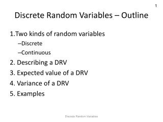
3) Random variables. A variable is something that can take different numeric values. A random variable (X) can take different numeric values with different probabilities. X is discrete if all its possible values can be listed. But if X can take any value in an interval like say [0,1], then X is continuous. Ex. Two cards are dealt to you. Let X be 1 if you get a pair, and X is 0 otherwise. P(X is 1) = 3/51 = 5.9% P(X is 0) = 94.1%. Ex. A coin is flipped, and X=20 if heads, X=10 if tails. The distribution of X means all the information about all the possible values X can take, along with their probabilities.
4) cdf, pmf, and density (pdf). Any random variable has a cumulative distribution function (cdf): F(b) = P(X < b). If X is discrete, then it has a probability mass function (pmf): f(b) = P(X = b). Continuous random variables are often characterized by their probability density functions (pdf, or density): a function f(x) such that P(X is in B) = ∫B f(x) dx .
6) Expected Value. For a discrete random variable X with pmf f(b), the expected value of X is the sum ∑ b f(b). The sum is over all possible values of b. (We’ll discuss continuous random variables later…) The expected value is also called the mean and denoted E(X) or m. Ex: 2 cards are dealt to you. X = 1 if pair, 0 otherwise. P(X is 1) = 3/51 = 5.9%, P(X is 0) = 94.1%. E(X) = (1 x 5.9%) + (0 x 94.1%) = 5.9%, or 0.059. Ex. Coin, X=20 if heads, X=10 if tails. E(X) = (20x50%) + (10x50%) = 15. Ex. Lotto ticket. f($10million) = 1/choose(52,6) = 1/20million, f($0) = 1-1/20mil. E(X) = ($10mil x 1/20million) = $0.50. The expected value of X represents a best guess of X. Compare with the sample mean, x = (X1 + X1 + … + Xn) / n.
Some reasons why Expected Value applies to poker: • Tournaments: some game theory results suggest that, in symmetric, winner-take-all games, the optimal strategy is the one which uses the myopic rule: that is, given any choice of options, always choose the one that maximizes your expected value. • Laws of large numbers: Some statistical theory (which we’ll get to later in this course) indicates that, if you repeat an experiment over and over repeatedly, your long-term average will ultimately converge to the expected value. So again, it makes sense to try to maximize expected value when playing poker (or making deals). • Checking results: A great way to check whether you are a long-term winning or losing player, or to verify if a certain strategy works or not, is to check whether the sample mean is positive and to see if it has converged to the expected value. (We will discuss this more later, too.)
Dan Harrington says that, with a hand like AA, you really want to be one-on-one. True or false? * Best possible pre-flop situation is to be all in with AA vs A8, where the 8 is the same suit as one of your aces, in which case you're about 94% to win. (the 8 could equivalently be a 6,7, or 9.) If you are all in for $100, then your expected holdings afterwards are $188. 1) In a more typical situation: you have AA and are up against TT. You're 80% to win, so your expected value is $160. 2) Suppose that, after the hand vs TT, you get QQ and get up against someone with A9 who has more chips than you do. The chance of you winning this hand is 72%, and the chance of you winning both this hand and the hand above is 58%, so your expected holdings after both hands are $232: you have 58% chance of having $400, and 42% chance to have $0. 3) Now suppose instead that you have AA and are all in against 3 callers with A8, KJ suited, and 44. Now you're 58.4% to quadruple up. So your expected holdings after the hand are $234, and the situation is just like (actually slightly better than) #1 and #2 combined: 58.4% chance to hold $400, and 41.6% chance for $0. * So, being all-in with AA against 3 players is much better than being all-in with AA against one player: in fact, it's about like having two of these lucky one-on-one situations.
What about with a low pair? 1) You have $100 and 55 and are up against A9. You are 56% to win, so your expected value is $112. 2) You have $100 and 55 and are up against A9, KJ, and QJs. Seems pretty terrible, doesn't it? But your odds are 27.3% to quadruple, so your expected value is $109. About the same as #1!
What about with KK? • 1) You have $100 and KK and are all-in against TT. You're 81% to double up, so your expected number of chips after the hand is $162. • 2) You have $100 and KK and are all-in against A9 and TT. You're 58% to have $300, so your expected value is $174. • So, if you have KK and an opponent with TT has already called you, and another who has A9 is thinking about whether to call you too, you actually want A9 to call! • Given this, one may question Harrington's suggested strategy of raising huge in order to isolate yourself against one player.