Operational Decision-Making Tools: Transportation and Transshipment Models
830 likes | 1.8k Vues
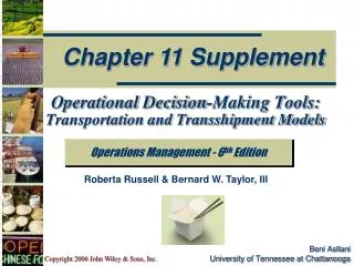
Chapter 11 Supplement. Operational Decision-Making Tools: Transportation and Transshipment Models. Beni Asllani University of Tennessee at Chattanooga. Operations Management - 6 hh Edition. Roberta Russell & Bernard W. Taylor, III. Just how do you make decisions?. Emotional direction

Operational Decision-Making Tools: Transportation and Transshipment Models
E N D
Presentation Transcript
Chapter 11 Supplement Operational Decision-Making Tools: Transportation and Transshipment Models Beni AsllaniUniversity of Tennessee at Chattanooga Operations Management - 6hh Edition Roberta Russell & Bernard W. Taylor, III Copyright 2006 John Wiley & Sons, Inc.
Just how do you make decisions? Emotional direction Intuition Analytic thinking Are you an intuit, an analytic, what??? How many of you use models to make decisions?? Copyright 2006 John Wiley & Sons, Inc.
Problems • Arise whenever there is a perceived difference between what is desired and what is in actuality. • Problems serve as motivators for doing something • Problems lead to decisions 42
Problem Problem MS Model Mental Model Mental Model Decision Decision Action Action Copyright 2006 John Wiley & Sons, Inc.
Model Classification Criteria • Purpose • Perspective • Use the perspective of the targeted decision-maker • Degree of Abstraction • Content and Form • Decision Environment • {This is what you should start any modeling facilitation meeting with} Copyright 2006 John Wiley & Sons, Inc.
Purpose • Planning • Forecasting • Training • Behavioral research Copyright 2006 John Wiley & Sons, Inc.
Perspective • Descriptive • “Telling it like it is” • Most simulation models are of this type • Prescriptive • “Telling it like it should be” • Most optimization models are of this type Copyright 2006 John Wiley & Sons, Inc.
Degree of Abstraction • Isomorphic • One-to-one • Homomorphic • One-to-many Copyright 2006 John Wiley & Sons, Inc.
Content and Form • verbal descriptions • mathematical constructs • simulations • mental models • physical prototypes Copyright 2006 John Wiley & Sons, Inc.
Decision Environment • Decision Making Under Certainty • TOOL: all of mathematical programming • Decision Making under Risk and Uncertainty • TOOL: Decision analysis--tables, trees, Bayesian revision • Decision Making Under Change and Complexity • TOOL: Structural models, simulation models Copyright 2006 John Wiley & Sons, Inc.
Mathematical Programming • Linear programming • Integer linear programming • some or all of the variables are integer variables • Network programming (produces all integer solutions) • Nonlinear programming • Dynamic programming • Goal programming • The list goes on and on • Geometric Programming Copyright 2006 John Wiley & Sons, Inc.
A Model of this class • What would we include in it? Copyright 2006 John Wiley & Sons, Inc.
Management Science Models • A QUANTITATIVE REPRESENTATION OF A PROCESS THAT CONSISTS OF THOSE COMPONENTS THAT ARE SIGNIFICANT FOR THE PURPOSE BEING CONSIDERED Copyright 2006 John Wiley & Sons, Inc.
Mathematical programming models covered in Ch 11, Supplement • Transportation Model • Transshipment Model Not included are: Shortest Route Minimal Spanning Tree Maximal flow Assignment problem many others Copyright 2006 John Wiley & Sons, Inc.
Transportation Model • A transportation model is formulated for a class of problems with the following characteristics • a product is transported from a number of sources to a number of destinations at the minimum possible cost • each source is able to supply a fixed number of units of product • each destination has a fixed demand for the product • Solution (optimization) Algorithms • stepping-stone • modified distribution • Excel’s Solver Copyright 2006 John Wiley & Sons, Inc.
Transportation Method: Example Copyright 2006 John Wiley & Sons, Inc.
Transportation Method: Example Copyright 2006 John Wiley & Sons, Inc.
Problem Formulation Using Excel Total Cost Formula Copyright 2006 John Wiley & Sons, Inc.
Using Solver from Tools Menu Copyright 2006 John Wiley & Sons, Inc.
Solution Copyright 2006 John Wiley & Sons, Inc.
Modified Problem Solution Copyright 2006 John Wiley & Sons, Inc.
The Underlying Network Copyright 2006 John Wiley & Sons, Inc.
For problems in which there is an underlying network: • There are easy (fast) solutions • An exception is the traveling salesman problem • The solutions are always integer ones • {How about solving a 50,000 node problem in less than a minute on a laptop??} Copyright 2006 John Wiley & Sons, Inc.
CARLTON PHARMACEUTICALS • Carlton Pharmaceuticals supplies drugs and other medical supplies. • It has three plants in: Cleveland, Detroit, Greensboro. • It has four distribution centers in: Boston, Richmond, Atlanta, St. Louis. • Management at Carlton would like to ship cases of a certain vaccine as economically as possible. Copyright 2006 John Wiley & Sons, Inc.
Data • Unit shipping cost, supply, and demand • Assumptions • Unit shipping cost is constant. • All the shipping occurs simultaneously. • The only transportation considered is between sources and destinations. • Total supply equals total demand. Copyright 2006 John Wiley & Sons, Inc.
Destinations Boston Sources 35 Cleveland 30 Richmond 40 S1=1200 32 37 40 Detroit 42 25 S2=1000 Atlanta 35 15 20 St.Louis Greensboro 28 S3= 800 D1=1100 NETWORK REPRESENTATION D2=400 D3=750 D4=750 Copyright 2006 John Wiley & Sons, Inc.
The Associated Linear Programming Model • The structure of the model is: Minimize <Total Shipping Cost> ST [Amount shipped from a source] = [Supply at that source] [Amount received at a destination] = [Demand at that destination] • Decision variables Xij = amount shipped from source i to destination j. where: i=1 (Cleveland), 2 (Detroit), 3 (Greensboro) j=1 (Boston), 2 (Richmond), 3 (Atlanta), 4(St.Louis) Copyright 2006 John Wiley & Sons, Inc.
Supply from Cleveland X11+X12+X13+X14 = 1200 Supply from Detroit X21+X22+X23+X24 = 1000 Supply from Greensboro X31+X32+X33+X34 = 800 X11 Cleveland X12 X31 S1=1200 X21 X13 X14 X22 X32 Detroit X23 S2=1000 X24 X33 Greensboro S3= 800 X34 The supply constraints Boston D1=1100 Richmond D2=400 Atlanta D3=750 St.Louis D4=750 Copyright 2006 John Wiley & Sons, Inc.
The complete mathematical programming model = = = = = = = Copyright 2006 John Wiley & Sons, Inc.
Excel Optimal Solution Copyright 2006 John Wiley & Sons, Inc.
Range of optimality WINQSB Sensitivity Analysis If this path is used, the total cost will increase by $5 per unit shipped along it Copyright 2006 John Wiley & Sons, Inc.
Range of feasibility Shadow prices for warehouses - the cost resulting from 1 extra case of vaccine demanded at the warehouse Shadow prices for plants - the savings incurred for each extra case of vaccine available at the plant Copyright 2006 John Wiley & Sons, Inc.
Transshipment Model Copyright 2006 John Wiley & Sons, Inc.
Transshipment Model: Solution Copyright 2006 John Wiley & Sons, Inc.
Copyright 2006 John Wiley & Sons, Inc.All rights reserved. Reproduction or translation of this work beyond that permitted in section 117 of the 1976 United States Copyright Act without express permission of the copyright owner is unlawful. Request for further information should be addressed to the Permission Department, John Wiley & Sons, Inc. The purchaser may make back-up copies for his/her own use only and not for distribution or resale. The Publisher assumes no responsibility for errors, omissions, or damages caused by the use of these programs or from the use of the information herein. Copyright 2006 John Wiley & Sons, Inc.
DEPOT MAX A General Network Problem • Depot Max has six stores. • Stores 5 and 6 are running low on the model 65A Arcadia workstation, and need a total of 25 additional units. • Stores 1 and 2 are ordered to ship a total of 25 units to stores 5 and 6. • Stores 3 and 4 are transshipment nodes with no demand or supply of their own. Copyright 2006 John Wiley & Sons, Inc.
Other restrictions • There is a maximum limit for quantities shipped on various routes. • There are different unit transportation costs for different routes. • Depot Max wishes to transport the available workstations at minimum total cost. Copyright 2006 John Wiley & Sons, Inc.
DATA: 20 10 7 1 3 5 Arcs: Upper bound and lower bound constraints: 6 5 12 11 7 2 4 6 15 15 • Supply nodes: Net flow out of the node] = [Supply at the node] • X12 + X13 + X15 - X21 = 10 (Node 1)X21 + X24 - X12 = 15 (Node 2) Network presentation • Intermediate transshipment nodes: [Total flow out of the node] = [Total flow into the node] • X34+X35 = X13 (Node 3)X46 = X24 + X34 (Node 4) Transportation unit cost • Demand nodes:[Net flow into the node] = [Demand for the node] • X15 + X35 +X65 - X56 = 12 (Node 5)X46 +X56 - X65 = 13 (Node 6) Copyright 2006 John Wiley & Sons, Inc.
The Complete mathematical model Copyright 2006 John Wiley & Sons, Inc.
WINQSB Input Data Copyright 2006 John Wiley & Sons, Inc.
WINQSB Optimal Solution Copyright 2006 John Wiley & Sons, Inc.
MONTPELIER SKI COMPANY Using a Transportation model for production scheduling • Montpelier is planning its production of skis for the months of July, August, and September. • Production capacity and unit production cost will change from month to month. • The company can use both regular time and overtime to produce skis. • Production levels should meet both demand forecasts and end-of-quarter inventory requirement. • Management would like to schedule production to minimize its costs for the quarter. Copyright 2006 John Wiley & Sons, Inc.
Data: • Initial inventory = 200 pairs • Ending inventory required =1200 pairs • Production capacity for the next quarter = 400 pairs in regular time. = 200 pairs in overtime. • Holding cost rate is 3% per month per ski. • Production capacity, and forecasted demand for this quarter (in pairs of skis), and production cost per unit (by months) Copyright 2006 John Wiley & Sons, Inc.
Initial inventory • Analysis of Unit costs • Unit cost = [Unit production cost] + • [Unit holding cost per month][the number of months stays in inventory] • Example: A unit produced in July in Regular time and sold in September costs 25+ (3%)(25)(2 months) = $26.50 • Analysis of demand: • Net demand to satisfy in July = 400 - 200 = 200 pairs • Net demand in August = 600 • Net demand in September = 1000 + 1200 = 2200 pairs • Analysis of Supplies: • Production capacities are thought of as supplies. • There are two sets of “supplies”: • Set 1- Regular time supply (production capacity) • Set 2 - Overtime supply Forecasted demand In house inventory Copyright 2006 John Wiley & Sons, Inc.
Network representation Production Month/period Month sold July R/T July R/T 25 25.75 26.50 0 1000 200 July July O/T 30 30.90 31.80 0 500 +M 26 26.78 0 +M +M 37 0 +M +M 29 0 Aug. R/T 600 +M 32 32.96 0 Aug. 800 Demand Production Capacity Aug. O/T 400 2200 Sept. Sept. R/T 400 Dummy 300 Sept. O/T 200 Copyright 2006 John Wiley & Sons, Inc.
Source: July production in R/T Destination: July‘s demand. Source: Aug. production in O/T Destination: Sept.’s demand Unit cost= $25 (production) 32+(.03)(32)=$32.96 Unit cost =Production+one month holding cost Copyright 2006 John Wiley & Sons, Inc.
Summary of the optimal solution • In July produce at capacity (1000 pairs in R/T, and 500 pairs in O/T). Store 1500-200 = 1300 at the end of July. • In August, produce 800 pairs in R/T, and 300 in O/T. Store additional 800 + 300 - 600 = 500 pairs. • In September, produce 400 pairs (clearly in R/T). With 1000 pairs retail demand, there will be (1300 + 500) + 400 - 1000 = 1200 pairs available for shipment to Ski Chalet. Inventory + Production - Demand Copyright 2006 John Wiley & Sons, Inc.
Problem 4-25 Copyright 2006 John Wiley & Sons, Inc.