Chapter 7: Transportation, assignment and transshipment problems
Chapter 7: Transportation, assignment and transshipment problems. Consists of nodes representing a set of origins and a set of destinations . An arc is used to represent the route from each origins to each destinations. Each origin has a supply and each destination has a demand.

Chapter 7: Transportation, assignment and transshipment problems
E N D
Presentation Transcript
Chapter 7:Transportation, assignment and transshipment problems
Consists of nodes representing a set of origins and a set of destinations. An arc is used to represent the route from each origins to each destinations. Each origin has a supply and each destination has a demand. Objective: To determine the optimal amount to ship from each origin to each destination Network flow model
Network flow problems Transportation Problem Assignment Problem Transshipment Problem
Transportation Problem Problems of distributing goods and services from several supply location to several demand locations Supply locations are called as Origin Demand locations are called as Destination Quantity of goods at origin are limited Quantity of goods at destinations are known Transportation Problem
Transportation Problem Each origin and destinations are represented by Circles called as nodes Each origin and destinations are connected by arc Each node requires one constraint Each arc requires one variable The sum of variables corresponding to arcs from an origin node must be less than or equal to origin supply. (Rule 3) The sum of variables corresponding to arcs into an destination node must equal to destination ‘s demand (Rule 4) Transportation Problem
Transportation Problem • The transportation problem seeks to minimize the total shipping costs of transporting goods from m origins (each with a supply si) to n destinations (each with a demand dj), when the unit shipping cost from an origin, i, to a destination, j, is cij. • The network representation for a transportation problem with two sources and three destinations is given on the next slide.
Transportation Problem • Network Representation 1 d1 c11 1 c12 s1 c13 2 d2 c21 c22 2 s2 c23 3 d3 SOURCES DESTINATIONS
Transportation Problem • LP Formulation The LP formulation in terms of the amounts shipped from the origins to the destinations, xij, can be written as: Min cijxij i j s.t. xij<si for each origin i j xij = dj for each destination j i xij> 0 for all i and j
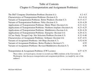
Distribution of goods from three plants to four distributions Supply Transportation problem Demands
Objectives To determine the routes to be used and quantity to be shipped from each origin to demand route that will provide minimum total transportation cost. Construct a network graph Connect each origin with the destination with arcs representing the routes between origin and the destinations. 12 Possible Routes Transportation Problem
7 Transportation network Boston 3 Cleveland 2 7 2 Chicago Bedford 5 S.Louis 5 6 2 Supplies York 4 Demands Lexington 3 5 Transportation Cost per unit
X ijnumber of units shipped from origin I to destination j X11 number of units shipped from origin (Cleveland) to destination 1 (boston) X12 number of units shipped from origin (Cleveland) to destination 2 (Chicago) Cost per unit Formulating the problem Objective Function=sum of cost from each source to destinations
Transportation cost shipped from Cleveland 3x11+2x12+7x13+6x14 Transportation cost shipped from Bedford 7x21+5x22+2x23+3x24 Transportation cost shipped from York 2x31+5x32+4x33+5x34 How many total variables and constraint?? What are supply and demand constraints???
Transportation shipped from Cleveland X11+x12+x13+x14<= 5000 Transportation shipped from Bedford X21+x22+x23+x24<=6000 Transportation shipped from York X31+x32+x33+x34<=2500 Supply constraint (Rule 3)
Transportation To boston X11+x21+x31= 6000 Transportation to Chicago X12+x22+x32=4000 Transportation to St.Louis X13+x23+x33=2500 Transportation to Lexington X14+x24+x34=1500 Objective function???? demand constraint (rule 4)
Objective function Min 3x11+2x12+7x13+6x14+7x21+5x22+2x23+3x24+2x31+5x32+4x33+5x34 S.T X11+x12+x13+x14 <= 5000 X21+x22+x23+x24 <=6000 X31+x32+x33+x34<=2500 X11 +x21 +x31 = 6000 X12 +x22 +x32 =4000 X13 +x23 +x33 =2500 X14 +x24 +x34 =1500 Model formalation
Solution Minimum total transportation cost? Units shipped=3500;cost per unit=3 Total cost from Cleveland to Boston??
General Linear Programming Model of Transportation problem Xij=number of units shipped from origin I to destination j Cij = cost per unit shipping from origin I to destination j Si= supply or capacity in units at origin I Dj= demand in units at destinations j
Generalized Assignment problem • Assigning jobs to machine • Agents to tasks • Sales personnel to sales territory • One to one assignment, i.e. one agent is assigned to one and only one task
Assignment Problem • An assignment problem seeks to minimize the total cost assignment of m workers to m jobs, given that the cost of worker i performing job j is cij. • It assumes all workers are assigned and each job is performed. • An assignment problem is a special case of a transportation problem in which all supplies and all demands are equal to 1; hence assignment problems may be solved as linear programs.
Assignment Problem • Network Representation c11 1 1 c12 c13 AGENTS TASKS c21 c22 2 2 c23 c31 c32 3 3 c33
Assignment Problem • LP Formulation Min cijxij i j s.t. xij = 1 for each agent i j xij = 1 for each task j i xij = 0 or 1 for all i and j • Note: A modification to the right-hand side of the first constraint set can be made if a worker is permitted to work more than 1 job.
Assignment Problem • LP Formulation Special Cases • Number of agents exceeds the number of tasks: xij< 1 for each agent i j • Number of tasks exceeds the number of agents: • Add enough dummy agents to equalize the • number of agents and the number of tasks. • The objective function coefficients for these • new variable would be zero.
Agent Task Problem Estimated project completion Time
7 Assignment problem network Client 1 Terry 10 9 15 Carle Client 2 18 5 6 6 14 Jack Client 3 Demands Supplies 3 Number of Constraints=6;Number of variables=9 Completion Time in Days
Days requires for Terry’s assignment 10x11+15x12+9x13 Days required for Carle ‘s assignment 9x21+18x22+5x23 Days required for Jack ‘s assignment 6x31+14x32+3x33 Objective Function Min10x11+15x12+9x13 +10x11+15x12+9x13+ 6x31+14x32+3x33 Problem formulation
Each project leader can be assigned to at most one client. X11+x12+x13 <=1 ;Terry ‘s assignment X21+x21+x23<=1; Carle ‘s assignment X31+X21 +x31<=1 ;Jack assignment Each Client must have at least one leader X11+X21+X31=1; Client 1 X12+X22+X32=1; Client 2 X13+X23+X33=1 ; Client 3 Constraint
Solution Terry is assigned to client2;x12=1 Carle is assigned to client3;x23=1 Jack is assigned to client 1 x31=1 Total completion time required is 26 days
Example: Hungry Owner A contractor pays his subcontractors a fixed fee plus mileage for work performed. On a given day the contractor is faced with three electrical jobs associated with various projects. Given below are the distances between the subcontractors and the projects. Projects SubcontractorABC Westside 50 36 16 Federated 28 30 18 Goliath 35 32 20 Universal 25 25 14 How should the contractors be assigned to minimize total costs?
Example: Hungry Owner • Network Representation 50 West. A 36 16 Subcontractors Projects 28 30 Fed. B 18 32 35 Gol. C 20 25 25 Univ. 14
Example: Hungry Owner • Linear Programming Formulation Min 50x11+36x12+16x13+28x21+30x22+18x23 +35x31+32x32+20x33+25x41+25x42+14x43 s.t. x11+x12+x13 < 1 x21+x22+x23 < 1 x31+x32+x33 < 1 x41+x42+x43 < 1 x11+x21+x31+x41 = 1 x12+x22+x32+x42 = 1 x13+x23+x33+x43 = 1 xij = 0 or 1 for all i and j Agents Tasks
Hungarian Method • Step 1: For each row, subtract the minimum number in that row from all numbers in that row. • Step 2:For each column, subtract the minimum number in that column from all numbers in that column. • Step 3:Draw the minimum number of lines to cover all zeroes. If this number = m, STOP -- an assignment can be made. • Step 4:Subtract d (the minimum uncovered number) from uncovered numbers. Add d to numbers covered by two lines. Numbers covered by one line remain the same. Then, GO TO STEP 3.
Hungarian Method • Finding the Minimum Number of Lines and Determining the Optimal Solution • Step 1:Find a row or column with only one unlined zero and circle it. (If all rows/columns have two or more unlined zeroes choose an arbitrary zero.) • Step 2:If the circle is in a row with one zero, draw a line through its column. If the circle is in a column with one zero, draw a line through its row. One approach, when all rows and columns have two or more zeroes, is to draw a line through one with the most zeroes, breaking ties arbitrarily. • Step 3:Repeat step 2 until all circles are lined. If this minimum number of lines equals m, the circles provide the optimal assignment.
Example: Hungry Owner • Initial Tableau Setup Since the Hungarian algorithm requires that there be the same number of rows as columns, add a Dummy column so that the first tableau is: ABCDummy Westside 50 36 16 0 Federated 28 30 18 0 Goliath 35 32 20 0 Universal 25 25 14 0
Example: Hungry Owner • Step 1:Subtract minimum number in each row from all numbers in that row. Since each row has a zero, we would simply generate the same matrix above. • Step 2:Subtract the minimum number in each column from all numbers in the column. For A it is 25, for B it is 25, for C it is 14, for Dummy it is 0. This yields: ABCDummy Westside 25 11 2 0 Federated 3 5 4 0 Goliath 10 7 6 0 Universal 0 0 0 0
Example: Hungry Owner • Step 3:Draw the minimum number of lines to cover all zeroes. Although one can "eyeball" this minimum, use the following algorithm. If a "remaining" row has only one zero, draw a line through the column. If a remaining column has only one zero in it, draw a line through the row. ABCDummy Westside 25 11 2 0 Federated 3 5 4 0 Goliath 10 7 6 0 Universal 0 0 0 0
Example: Hungry Owner • Step 3: Draw the minimum number of lines to cover all zeroes. ABCDummy Westside 23 9 0 0 Federated 1 3 2 0 Goliath 8 5 4 0 Universal 0 0 0 2
Example: Hungry Owner • Step 4:The minimum uncovered number is 1. Subtract 1 from uncovered numbers. Add 1 to numbers covered by two lines. This gives: ABCDummy Westside 23 9 0 1 Federated 0 2 1 0 Goliath 7 4 3 0 Universal 0 0 0 3
Example: Hungry Owner • Step 3:The minimum number of lines to cover all 0's is four. Thus, there is a minimum-cost assignment of 0's with this tableau. The optimal assignment is: SubcontractorProjectDistance Westside C 16 Federated A 28 Goliath (unassigned) Universal B 25 Total Distance = 69 miles
Transshipment Problem • Transshipment problems are transportation problems in which a shipment may move through intermediate nodes (transshipment nodes)before reaching a particular destination node. • Transshipment problems can be converted to larger transportation problems and solved by a special transportation program. • Transshipment problems can also be solved by general purpose linear programming codes. • The network representation for a transshipment problem with two sources, three intermediate nodes, and two destinations is shown on the next slide.
Transshipment Problem • Network Representation c36 3 c13 c37 1 6 s1 d1 c14 c46 c15 4 c47 Demand Supply c23 c56 c24 7 2 d2 s2 c25 5 c57 SOURCES INTERMEDIATE NODES DESTINATIONS
Contains three types of nodes: origin ,transhipment node and destination nodes For origin nodes sum of shipments out minus The sum of shipment in must be less than or equal to origin supply. For destination nodes sum of shipments out minus The sum of shipment in must be equal to demand For transhipment nodes the sum of shipments out must equal to sum of shipments in. Transhipment problem
Assignment problem network 5 Detroit 200 1 Denver 10 3 Kansas 600 6 Miami 150 4 Louisville 2 Atlanta 400 7 Dallas 350 Supplies Distribution Routes Demands 8 New Orleans 300 Number of Constraints=8;Number of variables=12
Origin Nodes ?? X13+X14 <=600 (Denver) X23+x24 <=400 (Atlanta) For transhipment Nodes x35+x36+x37+x38=x13+ x23 (Node 3;units in=units out) X45+X46+X47+X48=X14+X24(Node 4;units in= units out) For Destination nodes X35+x45=200 X36+x46=150 X37+x47=350 X38+x48=300 Constraints
Trasportion cost per unit Obj function 2x13+3x14+3x23+x24+2x35+6x36+3x37+6x38+4x45+4x46+6x47+5x48+4x28+x78
Solution Value of objective function?
Example: Transshipping Thomas Industries and Washburn Corporation supply three firms (Zrox, Hewes, Rockwright) with customized shelving for its offices. They both order shelving from the same two manufacturers, Arnold Manufacturers and Supershelf, Inc. Currently weekly demands by the users are 50 for Zrox, 60 for Hewes, and 40 for Rockwright. Both Arnold and Supershelf can supply at most 75 units to its customers. Additional data is shown on the next slide.
Example: Transshipping Because of long standing contracts based on past orders, unit costs from the manufacturers to the suppliers are: ThomasWashburn Arnold 5 8 Supershelf 7 4 The costs to install the shelving at the various locations are: ZroxHewesRockwright Thomas 1 5 8 Washburn 3 4 4
Example: Transshipping Zrox • Network Representation ZROX 50 1 5 Thomas Arnold 75 ARNOLD 5 8 8 Hewes 60 HEWES 3 7 Super Shelf Wash- Burn 4 75 WASH BURN 4 4 Rock- Wright 40
Example: Transshipping • Linear Programming Formulation • Decision Variables Defined xij = amount shipped from manufacturer i to supplier j xjk = amount shipped from supplier j to customer k where i = 1 (Arnold), 2 (Supershelf) j = 3 (Thomas), 4 (Washburn) k = 5 (Zrox), 6 (Hewes), 7 (Rockwright) • Objective Function Defined Minimize Overall Shipping Costs: Min 5x13 + 8x14 + 7x23 + 4x24 + 1x35 + 5x36 + 8x37 + 3x45 + 4x46 + 4x47