Signal & Linear system
Signal & Linear system. Chapter 4 Frequency - D omain Analysis : Laplace Transform Basil Hamed. 4.1 The Laplace Transform. Motivation for the Laplace Transform CT Fourier transform enables us to do a lot of things, e.g . Analyze frequency response of LTI systems Sampling Modulation

Signal & Linear system
E N D
Presentation Transcript
Signal & Linear system Chapter 4 Frequency - Domain Analysis : LaplaceTransform Basil Hamed
4.1 The Laplace Transform Motivation for the Laplace Transform • CT Fourier transform enables us to do a lot of things, e.g. • Analyze frequency response of LTI systems • Sampling • Modulation • Why do we need yet another transform? • One view of Laplace Transform is as an extension of the Fourier transform to allow analysis of broader class of signals and systems • In particular, Fourier transform cannot handle large (and important) classes of signals and unstable systems, i.e. when Basil Hamed
4.1 The Laplace Transform • The Laplace transform transforms the problem(D.EQ) from time domain to frequency domain. • Then the solution of the original D.EQ is arrived at, by obtaining the inverse transforms. • One of the problem that we faced using Fourier transform is many of the signals do not have Fourier transform.[ ex. exp(t)u(t), tu(t), and other time signals that are not absolutely integral] • The difficulty could be resolved by extending the Fourier transform so that x(t) is expressed as sum of complex exponentials, exp(-st) where Basil Hamed
4.1 The Laplace Transform exp(), exp( satisfies the absolute integrable For Ex. Given Find the frequency domain • Fourier Transform the Fourier transform does not exist. • Laplace Transform Basil Hamed
4.1 The Laplace Transform Laplace transform is the tool to map signals and system behavior from the time-domain into the frequency domain. For a signal x(t), its Laplace transform is defined by: • This general definite is known as two-sided (or bilateral) • Laplace Transform. Bilateral Basil Hamed
4.1 The Laplace Transform The one sided (unilateral) Laplace transform: Ex Given Find X(s) Solution • The above signal has Laplace transform only if thus • X(s) exists only if Basil Hamed
4.1 The Laplace Transform The range of values for the complex variable S for which the Laplace transform converges is called the Region of Convergence (ROC) Basil Hamed
4.1 The Laplace Transform Ex. Given Find X(s) Solution Note that X(s) for the two previous examples are the same the only distinguish is ROC Therefore, in order for the Laplace transform to be unique for each signal x(t). The ROC must be specified as part of the transform Basil Hamed
4.1 The Laplace Transform Basil Hamed
4.1 The Laplace Transform Ex. Given Find X(s) Solution -2<Re{s}<1 Re{s}>-2 Re{s}<1 Basil Hamed
4.1 The Laplace Transform Ex. Given Find X(s) Solution Ex. Find the Laplace transform of δ(t) and u(t). Basil Hamed
4.1 The Laplace Transform Ex. Find the Laplace transform of and cosω0t u(t). Basil Hamed
4.2 Properties of Laplace transform Ex. Find Laplace Transform of s Basil Hamed
4.2 Properties of Laplace transform Ex. Find X(s) Basil Hamed
4.2 Properties of Laplace transform Shifting in the S Domain Ex. Find • From Laplace Table we have Basil Hamed
4.2 Properties of Laplace transform Time Scaling Ex Find L{u()}, L{u()}=(1/) 1/s/ =1/s The result is expected, since u(t)=u(t) for>0 Differentiation & Integration in the Time Domain Basil Hamed
4.2 Properties of Laplace transform Ex. Find y(t) Solution Basil Hamed
4.2 Properties of Laplace transform Differentiation in The S-Domain Ex Given r(t)=t u(t), Find R(s) Solution R(s)=- Ex. Find • Solution Basil Hamed
4.2 Properties of Laplace transform Convolution • Then Ex given Find h(t) Solution Y(s)=X(s)H(s) H(s)=Y(s)/X(s) Basil Hamed
4.2 Properties of Laplace transform Initial-Value Theorem This property is useful, since it allows us to compute the initial value of the signal x(t) directly from the Laplace transform X(s) without having to find the inverse x(t) Ex Given Find x(0) Basil Hamed
4.2 Properties of Laplace transform Final-Value Theorem • Final-value Theorem exists only if the system is stable • Final-value Theorem is useful in many applications such as control theory, where we may need to find the final value(steady-state value) of the output of the system without solving for time domain Basil Hamed
4.2 Properties of Laplace transform Ex. Given Solution Ex. Given Solution System is unstable so there is no final value Basil Hamed
Stability Stability conditions for an LTIC system • Asymptotically stable if and only if all the poles of H(s) are in left-hand plane (LHP). The poles may be repeated or non-repeated. • Unstable if and only if either one or both of these conditions hold (i) at least one pole of H(s) is in right-hand plane (RHP) (ii) repeated poles of H(s) are on the imaginary axis • A system is said to be “marginally stable” if it has at least one distinct pole on the jω axis but no repeated poles on jω Marginally breaks Basil Hamed
Stability • In most applications we desire a stable system • We can easily check for stability by looking to see where the system’s poles are Example i. ii. Solution i. All poles are on LHP system is stable ii. One pole on RHP system is unstable Basil Hamed
Inverse Laplace Transform The function X(s) has to be a proper rational function to find the inverse of Laplace transform. The basic procedure is to express X(s) as a summation of terms whose inverse Laplace transform are available in a table. There are four general forms of solving the partial fraction; the roots of D(s) are either: • Real and Distinct • Complex and Distinct • Real and Repeated • Complex and Repeated Basil Hamed
Inverse Laplace Transform Real simple Poles Ex. Find x(t) Solution: Basil Hamed
Inverse Laplace Transform Basil Hamed
Inverse Laplace Transform Repeated Real Poles Ex. Solution Basil Hamed
Inverse Laplace Transform Ex. find x(t) Solution Simple Complex Poles Basil Hamed
Inverse Laplace Transform Basil Hamed
Inverse Laplace Transform X(s) contains distinct complex roots: Basil Hamed
Inverse Laplace Transform Repeated Complex Poles Ex. Solution: Basil Hamed
Inverse Laplace Transform Basil Hamed
4.3 Solution of Differential & Integro-Differential Equations The Laplace transform of differential equation is an algebraic equation that can be readily solved for Y(s). Next we take the inverse Laplace transform of Y(s) to find the desired solution y(t) Basil Hamed
4.3 Solution of Differential & Integro-Differential Equations Example 4.10 P. 371 Solve the following second-order linear differential equation: y (0) = 2, (0) =1and input x (t ) =. Solution Laplace (Frequency) Domain Time Domain Basil Hamed
4.3 Solution of Differential & Integro-Differential Equations Basil Hamed
4.3 Solution of Differential & Integro-Differential Equations Zero-input & Zero-state Responses The Laplace transform method gives the total response, which include zero-input and zero state components. It is possible to separate the two components if we so desire. Let’s think about where the terms come from: Input term • Initial condition term Basil Hamed
4.3 Solution of Differential & Integro-Differential Equations Basil Hamed
4.4 Analysis of Electrical Networks How to compute T.F for circuit one way to find the T.F of the circuit is to compute its differential equation and then take its Laplace transform However, it is generally simpler to compute T.F directly. Transfer Function: T.F is defined as the s-domain ratio of the output to the input Output Input Basil Hamed
4.4 Analysis of Electrical Networks We’ve seen that the system output’s LT is: So, if the system is in zero-state then we only get the second term: ⇒System effect in zero-state case is completely set by the transfer function Basil Hamed
4.4 Analysis of Electrical Networks Poles and Zeros of a system Given a system with Transfer Function: We can factor B(s) and A(s): (Recall: A(s) = characteristic polynomial) Pole-Zero Plot This gives us a graphical view of the system’s behavior Basil Hamed
4.4 Analysis of Electrical Networks Example Basil Hamed
4.4 Analysis of Electrical Networks S- Domain Time Domain Basil Hamed
4.4 Analysis of Electrical Networks Example: given the Circuit shown , find y(t) Solution: Apply Laplace Transform The total voltage in the loop is Basil Hamed
4.4 Analysis of Electrical Networks Exercise 4.4-1P 482 Find the zero state response , if the input voltage is . Find TF, write differential eq relating to x(t) Solution Loop Eq; Gramer rule yields Basil Hamed
4.4 Analysis of Electrical Networks Exercise 4.4-4 P 482 Find the loop currents for the input x(t) as shown in Figure below Solution: The Loop Eq. are Basil Hamed
4.4 Analysis of Electrical Networks Gramer’s rule yields Basil Hamed
4.5 Block Diagrams • Large systems may consist of an enormous number of components or elements. Analyzing such systems all at once could be next to impossible. In such cases, it is convenient to represent a system by suitably interconnected subsystems. • Each subsystem can be characterized in terms of its input-output relationships. Basil Hamed
X(s) W(s) H(s) Y(s) X(s) H1(s) H2(s) Y(s) = X(s) H1(s)H2(s) Y(s) H1(s) = X(s) Y(s) X(s) H1(s) + H2(s) Y(s) H2(s) E(s) X(s) G(s) 1 + G(s)H(s) Y(s) X(s) G(s) Y(s) = - H(s) 4.5 Block Diagrams
4.5 Block Diagrams Example: A basic feedback system consisting of block find TF More on this later in Control Course feedback