Overview of Computer Vision Classification Techniques and Concepts
This course webpage outlines key concepts and techniques in computer vision classification, including image processing, motion estimation, and various learning paradigms. It covers unsupervised learning with clustering methods like k-means, and supervised learning including metrics for assessing classifier performance. Key topics include feature extraction, decision surfaces, and classifiers such as k-nearest neighbors and linear discriminants. Practical applications and the challenges of classification are also discussed, aiming to provide students with a comprehensive foundation in the field.


Overview of Computer Vision Classification Techniques and Concepts
E N D
Presentation Transcript
Vision Review:Classification Course web page: www.cis.udel.edu/~cer/arv October 3, 2002
Announcements • Homework 2 due next Tuesday • Project proposal due next Thursday, Oct. 10. Please make an appointment to discuss before then
Computer Vision Review Outline • Image formation • Image processing • Motion & Estimation • Classification
Outline • Classification terminology • Unsupervised learning (clustering) • Supervised learning • k-Nearest neighbors • Linear discriminants • Perceptron, Relaxation, modern variants • Nonlinear discriminants • Neural networks, etc. • Applications to computer vision • Miscellaneous techniques
Classification Terms • Data: A set of N vectors x • Features are parameters of x; x lives in feature space • May be whole, raw images; parts of images; filtered images; statistics of images; or something else entirely • Labels: C categories; each x belongs to some ci • Classifier: Create formula(s) or rule(s) that will assign unlabeled data to correct category • Equivalent definition is to parametrize a decision surface in feature space separating category members
Features and Labels for Road Classification • Feature vectors: 410 features/point over 32 x 20 grid • Color histogram[Swain & Ballard, 1991] (24 features) • 8 bins per RGB channel over surrounding 31 x 31 camera subimage • Gabor wavelets[Lee, 1996] (384) • Characterize texture with 8-bin histogram of filter responses for 2 phases, 3 scales, 8 angles over 15 x 15 camera subimage • Ground height, smoothness (2) • Mean, variance of laser height values projecting to 31 x 31 camera subimage • Labels derived from inside/ outside relationship of feature point to road-delimiting polygon 0° even 45° even 0° odd from Rasmussen, 2001
Key Classification Problems • What features to use? How do we extract them from the image? • Do we even have labels (i.e., examples from each category)? • What do we know about the structure of the categories in feature space?
Unsupervised Learning • May know number of categories C, but not labels • If we don’t know C, how to estimate? • Occam’s razor (formalized as Minimum Description Length, or MDL, principle): Favor simpler classifiers over more complex ones • Akaike Information Criterion (AIC) • Clustering methods • k-means • Hierarchical • Etc.
k-means Clustering • Initialization: Given k categories, N points. Pick k points randomly; these are initial means 1, …, k • (1) Classify N points according to nearest i • (2) Recompute mean i of each cluster from member points • (3) If any means have changed, goto (1)
Example: 3-means Clustering from Duda et al. Convergence in 3 steps
Supervised Learning:Assessing Classifier Performance • Bias: Accuracy or quality of classification • Variance: Precision or specificity—how stable is decision boundary for different data sets? • Related to generality of classification result Overfitting to data at hand will often result in a very different boundary for new data
Supervised Learning: Procedures • Validation: Split data into training and test set • Training set: Labeled data points used to guide parametrization of classifier • % misclassified guides learning • Test set: Labeled data points left out of training procedure • % misclassified taken to be overall classifier error • m-fold Cross-validation • Randomly split data into m equal-sized subsets • Train m times on m - 1 subsets, test on left-out subset • Error is mean test error over left-out subsets • Jackknife: Cross-validation with 1 data point left out • Very accurate; variance allows confidence measuring
k-Nearest Neighbor Classification • For a new point, grow sphere in feature space until k labeled points are enclosed • Labels of points in sphere vote to classify • Low bias, high variance: No structure assumed from Duda et al.
Linear Discriminants • Basic: g(x) = wTx + w0 • w is weight vector, x is data, w0 is bias or threshold weight • Number of categories • Two: Decide c1 if g(x) < 0, c2 if g(x) > 0. g(x) = 0 is decision surface—a hyperplane when g(x) linear • Multiple: Define C functions gi(x) = wTxi + wi0. Decide ci if gi(x) > gj(x) for all j i • Generalized: g(x) = aTy • Augmented form: y = (1, xT)T, a = (w0, wT)T • Functions yi = yi(x) can be nonlinear—e.g., y = (1, x, x2)T
Separating Hyperplane in Feature Space from Duda et al.
Computing Linear Discriminants • Linear separability: Some a exists that classifies all samples correctly • Normalization: If yi is classified correctly when aTyi < 0 and its label is c1, simpler to replace all c1-labeled samples with their negation • This leads to looking for an a such that aTyi > 0 for all of the data • Define a criterion function J(a) that is minimized if a is a solution. Then gradient descent on J (for example) leads to a discriminant
Criterion Functions • Idea: J = Number of misclassified data points. But only piecewise continuous Not good for gradient descent • Approaches • Perceptron: Jp(a) = yY (-aTy), where Y(a) is the set of samples misclassified by a • Proportional to sum of distances between misclassified samples and decision surface • Relaxation: Jr(a) = ½ yY (aTy - b)2 / ||y||2, where Y(a) is now set of samples such that aTy b • Continuous gradient; J not so flat near solution boundary • Normalize by sample length to equalize influences
Non-Separable Data: Error Minimization • Perceptron, Relaxation assume separability—won’t stop otherwise • Only focus on erroneous classifications • Idea: Minimize error over all data • Try to solve linear equations rather than linear inequalities: aTy = b Minimize i (aTyi – bi)2 • Solve batch with pseudoinverse or iteratively with Widrow-Hoff/LMS gradient descent • Ho-Kashyap procedure picks a and b together
Other Linear Discriminants • Winnow: Improved version of Perceptron • Error decreases monotonically • Faster convergence • Appropriate choice of b leads to Fisher’s Linear Discriminant (used in “Vision-based Perception for an Autonomous Harvester,” by Ollis & Stentz) • Support Vector Machines (SVM) • Map input nonlinearly to higher-dimensional space (where in general there is a separating hyperplane) • Find separating hyperplane that maximizes distance to nearest data point
Neural Networks • Many problems require a nonlinear decision surface • Idea: Learn linear discriminant and nonlinear mapping functions yi(x) simultaneously • Feedforward neural networks are multi-layer Perceptrons • Inputs to each unit are summed, bias added, put through nonlinear transfer function • Training: Backpropagation, a generalization of LMS rule
Neural Networks in Matlab net = newff(minmax(D), [h o], {'tansig', 'tansig'}, 'traincgf'); net = train(net, D, L); test_out = sim(net, testD); where: D is training data feature vectors (row vector) L is labels for training data testD is testing data feature vectors h is number of hidden units o is number of outputs
Dimensionality Reduction • Functions yi = yi(x) can reduce dimensionality of feature space More efficient classification • If chosen intelligently, we won’t lose much information and classification is easier • Common methods • Principal components analysis (PCA): Maximize total “scatter” of data • Fisher’s Linear Discriminant (FLD): Maximize ratio of between-class scatter to within-class scatter
Principal Component Analysis • Orthogonalize feature vectors so that they are uncorrelated • Inverse of this transformation takes zero mean, unit variance Gaussian to one describing covariance of data points • Distance in transformed space is Mahalanobis distance • By dropping eigenvectors of covariance matrix with low eigenvalues, we are essentially throwing away least important dimensions
Dimensionality Reduction: PCA vs. FLD from Belhumeur et al., 1996
Face Recognition(Belhumeur et al., 1996) • Given cropped images {I} of faces with different lighting, expressions • Nearest neighbor approach equivalent to correlation (I’s normalized to 0 mean, variance 1) • Lots of computation, storage • PCA projection (“Eigenfaces”) • Better, but sensitive to variation in lighting conditions • FLD projection (“Fisherfaces”) • Best (for this problem)
Bayesian Decision Theory: Classification with Known Parametric Forms • Sometimes we know (or assume) that the data in each category is drawn from a distribution of a certain form—e.g., a Gaussian • Then classification can be framed as simply a nearest-neighbor calculation, but with a different distance metric to each category—i.e., the Mahalanobis distance for Gaussians
Decision Surfaces for Various 2-Gaussian Situations from Duda et al.
Example:Color-based Image Comparison • Per image: e.g., histograms from Image Processing lecture • Per pixel: Sample homogeneously-colored regions… • Parametric: Fit model(s) to pixels, threshold on distance (e.g., Mahalanobis) • Non-parametric: Normalize accumulated array, threshold on likelihood
Color Similarity: RGB Mahalanobis Distance PCA-fitted ellipsoid Sample
Non-parametric Color Models courtesy of G. Loy Skin chrominance points Smoothed, [0,1]-normalized
Non-parametric Skin Classification courtesy of G. Loy
Other Methods • Boosting • AdaBoost (Freund & Schapire, 1997) • “Weak learners”: Classifiers that do better than chance • Train m weak learners on successive versions of data set with misclassifications from last stage emphasized • Combined classifier takes weighted average of m “votes” • Stochastic search (think particle filtering) • Simulated annealing • Genetic algorithms