COSC 3100 Divide and Conquer
470 likes | 744 Vues
COSC 3100 Divide and Conquer. Instructor: Tanvir. What is Divide and Conquer ?. 3 rd algorithm design technique, we are going to study Very important: two out of ten most influential algorithms in the twentieth century is based directly on “Divide and Conquer” technique

COSC 3100 Divide and Conquer
E N D
Presentation Transcript
COSC 3100Divide and Conquer Instructor: Tanvir
What is Divide and Conquer ? • 3rd algorithm design technique, we are going to study • Very important: two out of ten most influential algorithms in the twentieth century is based directly on “Divide and Conquer” technique • Quicksort (we shall study today) • Fast Fourier Transform (we shall not study in this course, but any “signal processing” course is based on this idea)
Divide and Conquer • Three steps are involved: • Divide the problem into several subproblems, perhaps of equal size • Subproblems are solved, typically recursively • The solutions to the subproblems are combined to get a solution to the original problem Real work is done in 3 different places: in partitioning; at the very tail end of the recursion, when subproblems are so small that they are solved directly; and in gluing together of partial solutions
Divide and Conquer (contd.) Problem of size n Subproblem 1 of size n/2 Subproblem 2 of size n/2 Don’t assume always breaks up into 2, could be > 2 subproblems Solution to subproblem 1 Solution to subproblem 2 Solution to the original probelm
Divide and Conquer (contd.) • In “politics” divide and rule (latin: divide et impera) is a combination of political, military, and economic strategy of gaining and maintaining power by breaking up larger concentrations of power into chunks that individually have less power than the one who is implementing the strategy. (read more on wiki: “Divide and rule”)
Divide and Conquer (contd.) • Let us add n numbers using divide and conquer technique a0 + a1 + …… + an-1 a0 + …… + + …… + an-1 Is it more efficient than brute force ? Let’s see with an example
Div. & Conq. (add n numbers) # of additions is same as in brute force, needs stack for recursion… Bad! not all divide and conquer works!! Could be efficient for parallel processors though….
Div. & Conq. (contd.) • Usually in div. & conq., a problem instance of size n is divided into two instances of size n/2 • More generally, an instance of size n can be divided into b instances of size n/b, with a of them needing to be solved • Assuming that n is a power of b (n = bm), we get • T(n) = aT(n/b) + f(n) • Here, f(n) accounts for the time spent in dividing an instance of size n into subproblems of size n/b and combining their solution • For adding n numbers, a = b = 2 and f(n) = 1 general divide-and-conquer recurrence
Div & Conq. (contd.) What if a = 1? Have we seen it? • T(n) = aT(n/b)+f(n), a ≥ 1, b > 1 • Master Theorem: If f(n) єΘ(nd) where d ≥ 0 then So, A(n) єΘ() Or, A(n) єΘ(n) Θ(nd) if a < bd T(n) є Θ(ndlgn) if a = bd Without going through back-subs. we got it, but not quite… Θ() if a > bd For adding n numbers with divide and conquer technique, the number of additions A(n) is: A(n) = 2A(n/2)+1 Here, a = ?, b = ?, d = ? a = 2, b = 2, d = 0 Which of the 3 cases holds ? a = 2 > bd= 20, case 3
Div. & Conq. (contd.) T(n) = aT(n/b)+f(n), a ≥ 1, b > 1 If f(n) єΘ(nd) where d ≥ 0, then T(n) = 2T(n/2)+6n-1? T(n) = 3 T(n/2) + n a = 3, b = 2, f(n) єΘ(n1), so d = 1 Θ(nd) if a < bd Case 3: T(n) єΘ( ) = Θ( ) a=3 > bd=21 T(n) є Θ(ndlgn) if a = bd T(n) = 3 T(n/2) + n2 a = 3, b = 2, f(n) єΘ(n2), so d = 2 Case 1: T(n) єΘ( ) a=3 < bd=22 Θ() if a > bd T(n) = 4 T(n/2) + n2 a = 4, b = 2, f(n) єΘ(n2), so d = 2 Case 2: T(n) єΘ( lgn ) a=4 = bd=22 T(n) = 0.5 T(n/2) + 1/n Master thm doesn’t apply,a<1, d<0 Master thm doesn’t apply f(n) not polynomial T(n) = 2 T(n/2) + n/lgn f(n) is not positive, doesn’t apply T(n) = 64 T(n/8) – n2lgn T(n) = 2n T(n/8) + n a is not constant, doesn’t apply
Div. & Conq.: Mergesort A[0……n-1] • Sort an array A[0..n-1] divide A[0……] A[……n-1] sort sort A[……n-1] A[0……] merge A[0……n-1] Go on dividing recursively…
Div. & Conq.: Mergesort(contd.) ALGORITHMMergesort(A[0..n-1]) //sorts array A[0..n-1] by recursive mergesort //Input: A[0..n-1] to be sorted //Output: Sorted A[0..n-1] if n > 1 copy A[0..-1] to B[0.. -1] copy A[..n-1] to C[0..-1] Mergesort(B[0..-1]) Mergesort(C[0..-1]) Merge(B, C, A) B: C: 1 2 3 4 5 7 8 9 A:
Div. & Conq.: Mergesort(contd.) ALGORITHM Merge(B[0..p-1], C[0..q-1], A[0..p+q-1]) //Merges two sorted arrays into one sorted array //Input: Arrays B[0..p-1] and C[0..q-1] both sorted //Output: Sorted array A[0..p+q-1] of elements of B and C i <- 0; j <- 0; k <- 0; whilei < p and j < q do if B[i] ≤ C[j] A[k] <- B[i]; i <- i+1 else A[k] <- C[j]; j <- j+1 k <- k+1 ifi = p copy C[j..q-1] to A[k..p+q-1] else copy B[i..p-1] to A[k..p+q-1]
Div. & Conq.: Mergesort(contd.) Divide: Merge:
Div. & Conq.: Mergesort(contd.) ALGORITHMMergesort(A[0..n-1]) //sorts array A[0..n-1] by recursive mergesort //Input: A[0..n-1] to be sorted //Output: Sorted A[0..n-1] if n > a copy A[0..-1] to B[0.. -1] copy A[..n-1] to C[0..-1] Mergesort(B[0..-1]) Mergesort(C[0..-1]) Merge(B, C, A) ALGORITHM Merge(B[0..p-1], C[0..q-1], A[0..p+q-1]) //Merges two sorted arrays into one sorted array //Input: Arrays B[0..p-1] and C[0..q-1] both sorted //Output: Sorted array A[0..p+q-1] of elements of B //and C i <- 0; j <- 0; k <- 0; whilei < p and j < q do if B[i] ≤ C[j] A[k] <- B[i]; i <- i+1 else A[k] <- C[j]; j <- j+1 k <- k+1 ifi = p copy C[j..q-1] to A[k..p+q-1] else copy B[i..p-1] to A[k..p+q-1] What is the time-efficiency of Meresort? Input size: n = 2m Basic op: comparison C(n) depends on input type… C(n) = 2C(n/2) + CMerge(n) for n > 1, C(1) = 0 Cworst(n) = 2Cworst(n/2)+n-1 for n > 1 Cworst(1) = 0 B: C: In worst-case CMerge(n) = n-1 A: Cworst(n) = nlgn-n+1 єΘ(nlgn) How many comparisons is needed for this Merge? Could use the master thm too!
Div. & Conq.: Mergesort(contd.) • Worst-case of Mergesort is Θ(nlgn) • Average-case is also Θ(nlgn) • It is stable but quicksort and heapsort are not • Possible improvements • Implement bottom-up. Merge pairs of elements, merge the sorted pairs, so on… (does not require recursion-stack anymore) • Could divide into more than two parts, particularly useful for sorting large files that cannot be loaded into main memory at once: this version is called “multiwaymergesort” • Not in-place, needs linear amount of extra memory • Though we could make it in-place, adds a bit more “complexity” to the algorithm
Div. & Conq.: Quicksort • Another divide and conquer based sorting algorithm, discovered by C. A. R. Hoare (British) in 1960 while trying to sort words for a machine translation project from Russian to English • Instead of “Merge” in Mergesort, Quicksort uses the idea of partitioning which we already have seen with “Lomuto Partition”
Div. & Conqr.: Quicksort (contd.) A[0]…A[s-1] A[s] A[s+1]…A[n-1] A[0]…A[n-1] all are ≥ A[s] all are ≤ A[s] Notice: In Mergesort all work is in combining the partial solutions. In Quicksort all work is in dividing the problem, Combining does not require any work! A[s] is in it’s final position Now continue working with these two parts
Div. & Conqr.: Quicksort (contd.) ALGORITHM Quicksort(A[l..r]) //Sorts a subarray by quicksort //Input: Subarray of array A[0..n-1] defined by its //left and right indices l and r //Output: Subarray A[l..r] sorted in nondecreasing //order if l < r s <- Partition( A[l..r] ) // s is a split position Quicksort( A[l..s-1] ) Quicksort( A[s+1]..r )
Div. & Conqr.: Quicksort (contd.) • As a partition algorithm we could use “Lomuto Partition” • But we shall use the more sophisticated “Hoare Partition” instead • We start by selecting a “pivot” • There are various strategies to select the pivot, we shall use the simplest: we shall select pivot, p =A[l], the first element of A[l..r]
Div. & Conqr.: Quicksort (contd.) p ≥ p ≤ p p i j p If A[i] < p, we continue incrementing i, stop when A[i] ≥ p If A[j] > p, we continue decrementing j, stop when A[j] ≤ p j i p ≥ p ≤ p all ≥ p all ≤ p j i p ≤ p ≥ p all ≤ p all ≥ p j=i p = p all ≤ p all ≥ p
Div. & Conqr.: Quicksort (contd.) i could go out of array’s bound, we could check or we could put a “sentinel” at the end… ALGORITHMHoarePartition(A[l..r]) //Output: the split position p <- A[l] i <- l; j <- r+1 repeat repeat i <- i+1 until A[i] ≥ p repeat j <- j-1 until A[j] ≤ p swap( A[i], A[j] ) untili ≥ j swap( A[i], A[j] ) // undo last swap when i ≥ j swap( A[l], A[j] ) return j Do you see any possible problem with this pseudocode ? More sophisticated pivot selection that we shall see briefly makes this “sentinel” unnecessary…
Div. & Conqr.: Quicksort (contd.) j j i i j j i i j i j i j i i j j i i j i j j i j i i=j j i
Div. & Conqr.: Quicksort (contd.) l=2,r=1 l=0,r=7 l=5,r=5 l=0,r=0 l=3,r=3 l=7,r=7 l=2,r=3 l=5,r=7 l=0,r=3 s=2 s=4 s=1 s=6
Div. & Conqr.: Quicksort (contd.) ALGORITHM Quicksort(A[l..r]) if l < r s <- HoarePartition ( A[l..r] ) Quicksort( A[l..s-1] ) Quicksort( A[s+1]..r ) Time-complexity of this line ? i j • Let us analyze Quicksort So, n+1 comparisons when cross-over i j If all splits happen in the middle, it is the best-case! j i ALGORITHMHoarePartition(A[l..r]) //Output: the split position p <- A[l] i <- l; j <- r+1 repeat repeat i <- i+1 until A[i] ≥ p repeat j <- j-1 until A[j] ≤ p swap( A[i], A[j] ) untili ≥ j swap( A[i], A[j] ) // undo last swap when i ≥ j swap( A[l], A[j] ) return j So, n comparisons when coincide What if, i,j Cbest(n) = 2Cbest(n/2)+n for n > 1 Cbest(1) = 0
Div. & Conqr.: Quicksort (contd.) T(n) = aT(n/b)+f(n), a ≥ 1, b > 1 If f(n) єnd with d ≥ 0, then ALGORITHM Quicksort(A[l..r]) if l < r s <- Partition( A[l..r] ) Quicksort( A[l..s-1] ) Quicksort( A[s+1]..r ) j j j j Θ(nd) if a < bd i j 5+1=6 Θ(ndlgn) if a = bd T(n) є Cbest(n) = 2Cbest(n/2)+n for n > 1 Cbest(1) = 0 j i 4+1=5 Θ() if a > bd j i Using Master Thm, Cbest(n) єΘ(nlgn) 3+1=4 What is the worst-case ? j i 2+1=3 Cworst(n) = (n+1) + (n-1+1) + … + (2+1) = (n+1) + … + 3 = (n+1) + … + 3 + 2 + 1 – (2 + 1) = - 3 = - 3 єΘ(n2) ! So, Quicksort’s fate depends on its average-case!
Div. & Conqr.: Quicksort (contd.) ALGORITHM Quicksort(A[l..r]) if l < r s <- Partition( A[l..r] ) Quicksort( A[l..s-1] ) Quicksort( A[s+1]..r ) • Let us sketch the outline of average-case analysis… Cavg(n) is the average number of key-comparisons made by the Quicksort on a randomly ordered array of size n After n+1 comparisons, a partition can happen in any position s (0 ≤ s ≤ n-1) Let us assume that partition split can happen in each position s with equal probability 1/n After the partition, left part has s elements, Right part has n-1-s elements s 0 n-1 Cavg(n) = Expected[ Cavg(s) + Cavg(n-1-s) + (n+1) ] p Average over all possibilities s elements Cavg(n) = Cavg(0) = 0, Cavg(1) = 0 n-1-s elements Cavg(n) ≈ 1.39nlgn
Div. & Conqr.: Quicksort (contd.) • Recall that for Quicksort, Cbest(n) ≈ nlgn • So, Cavg(n) ≈ 1.39nlgn is not far from Cbest(n) • Quicksort is usually faster than Mergesort or Heapsort on randomly ordered arrays of nontrivial sizes • Some possible improvements • Randomized quicksort: selects a random element as pivot • Median-of-three: selects median of left-most, middle, and right-most elements as pivot • Switching to insertion sort on very small subarrays, or not sorting small subarrays at all and finish the algorithm with insertion sort applied to the entire nearly sorted array • Modify partitioning: three-way partition These improvements can speed up by 20% to 30%
Div. & Conqr.: Quicksort (contd.) • Weaknesses • Not stable • Requires a stack to store parameters of subarrays that are yet to be sorted, the stack can be made to be in O(lgn) but that is still worse than O(1) space efficiency of Heapsort DONE with Quicksort!
Div. & Conq. : Multiplication of Large Integers • We want to efficiently multiply two very large numbers, say each has more than 100 decimal digits • How do we usually multiply 23 and 14? • 23 = 2*101 + 3*100, 14 = 1*101 + 4*100 • 23*14 = (2*101 + 3*100) * (1*101 + 4*100) • 23*14 = (2*1)102 + (2*4+3*1)101+(3*4)100 • How many multiplications? 4 = n2
Div. & Conq. : Multiplication of Large Integers We can rewrite the middle term as: (2*4+3*1) = (2+3)*(1+4) - 2*1 - 3*4 • 23*14 = (2*1)102 + (2*4+3*1)101+(3*4)100 What has been gained? We have reused 2*1 and 3*4 and now need one less multiplication If we have a pair of 2-digits numbers a and b a = a1a0 and b = b1b0 we can write c = a*b = c2102+c1101+c0100 c0 = a0*b0 c2 = a1*b1 c1 = (a1+a0)*(b1+b0)-(c2+c0)
Div. & Conq. : Multiplication of Large Integers If we have a pair of 2-digits numbers a and b a = a1a0 and b = b1b0 we can write c = a*b = c2102+c1101+c0100 a = 1234 = 1*103+2*102+3*101+4*100 = (12)102+(34) c2 = a1*b1 , c0 = a0*b0 c1 = (a1+a0)*(b1+b0)-(c2+c0) (12)102+(34) = (1*101+2*100)102+3*101+4*100 If we have two n-digits numbers, a and b (assume n is a power of 2) Apply the same idea recursively to get c2, c1, c0 until n is so small that you can you can directly multiply a0 a1 a: n/2 digits b1 b0 b: c = a*b = = = We can write, a = a110n/2 + a0 Why? b = b110n/2 + b0 c0 = a0*b0 c2 = a1*b1 c1 = (a1+a0)*(b1+b0)-(c2+c0)
Div. & Conq. : Multiplication of Large Integers c = a*b = Notice: a1, a0, b1, b0 all are n/2 digits numbers 5 additions 1 subtraction c2 = a1*b1 c0 = a0*b0 So, computing a*b requires three n/2-digits multiplications c1 = (a1+a0)*(b1+b0)-(c2+c0) Recurrence for the number of Multiplications is M(n) = 3M(n/2) for n > 1 Assume n = 2m M(n) = 3M(n/2) = 3[ 3M(n/22) ] = 32M(n/22) M(n) = 3mM(n/2m) = ? M(1) = ? How many additions And subtractions? Let = x = = x = M(n) = 3m = 3lgn = nlg3 # of add/sub, A(n) = 3A(n/2)+cn for n > 1 A(1) = 0 Why? Using Master Thm, A(n) єΘ(nlg3) M(n) ≈ n1.585
Div. & Conq. : Multiplication of Large Integers • People used to believe that multiplying two n-digits number has complexity Ω(n2) • In 1960, Russian mathematician Anatoly Karatsuba, gave this algorithm whose asymptotic complexity is Θ(n1.585) • A use of large number multiplication is in modern cryptography • It does not generally make sense to recurse all the way down to 1 bit: for most processors 16- or 32-bit multiplication is a single operation; so by this time, the numbers should be handed over to built-in procedure Next we see how to multiply Matrices efficiently…
Div. & Conq. : Strassen’s Matrix Multiplication • 2 • 3 4 3 5 1 4 5 13 13 31 How many multiplications and additions did we need? • How do we multiply two 2×2 matrices ? = 8 mults and 4 adds V. Strassen in 1969 found out, he can do the above multiplication in the following way: m1+m4-m5+m7 m3+m5 m2+m4 m1+m3-m2+m6 c00 c01 c10 c11 a00 a01 a10 a11 b00 b01 b10 b11 = = m2 = (a10+a11)*b00 m1 = (a00+a11)*(b00+b11) m3 = a00*(b01-b11) 7 mults 18 adds/subs m4 = a11*(b10-b00) m5 = (a00+a01)*b11 m6 = (a10-a00)*(b00+b01) m7 = (a01-a11)*(b10+b11)
Div. & Conq. : Strassen’s Matrix Multiplication • Let us see how we can apply Strassen’s idea for multiplying two n×n matrices Let A and B be two n×n matrices where n is a power of 2 A00 A01 A10 A11 B00 B01 B10 B11 C00 C01 C10 C11 = Each block is (n/2)×(n/2) E.g., In Strassen’s method, M1 = (A00+A11)*(B00+B11) M2= (A10+A11)*B00 etc. You can treat blocks as if they were numbers to get the C = A*B
Div. & Conq. : Strassen’s Matrix Multiplication ALGORITHMStrassen(A, B, n) //Input: A and B are n×n matrices //where n is a power of two //Output: C = A*B if n = 1 return C = A*B else Partition A = and B = where the blocks Aij and Bij are (n/2)-by-(n/2) M1 <- Strassen(A00+A11, B00+B11, n/2) M2 <- Strassen(A10+A11, B00, n/2) M3 <- Strassen(A00, B01-B11, n/2) M4 <- Strassen(A11, B10-B00, n/2) M5 <- Strassen(A00+A01, B11, n/2) M6 <- Strassen(A10-A00, B00+B01, n/2) M7 <- Strassen(A01-A11, B10+B11, n/2) C00 <- M1+M4-M5+M7 C01 <- M3+M5 C10 <- M2+M4 C11 <- M1+M3-M2+M6 return C = Recurrence for # of multiplications is M(n) = 7M(n/2) for n > 1 M(1) = ? For n = 2m, M(n) = 7M(n/2) = 72M(n/22) B00 B01 B10 B11 A00 A01 A10 A11 M(n) = 7m M(n/2m) = 7m = 7lgn = nlg7 ≈ n2.807 For # of adds/subs, A(n) = 7A(n/2)+18(n/2)2 for n > 1 A(1) = 0 Using Master thm, A(n) єΘ(nlg7) better than brute-force’s Θ(n3) C00 C01 C10 C11 DONE WITH STRASSEN!
Div. & Conq.: Closest pair ALGORITHMBruteForceClosestPair(P) //Input: A list P of n (n≥2) points p1(x1,y1), //p2(x2,y2), …, pn(xn,yn) //Output: distance between closest pair d <- ∞ fori <- 1 to n-1 do for j <- i+1 to n do d <- min( d, sqrt( ) ) return d • Find the two closest points in a set of n points Traffic Control: detect two vehicles most likely to collide Idea: consider each pair of points and keep track of the pair having the minimum distance n 2 = pairs, so time-efficiency is in Θ(n2) There are
Div. & Conq.: Closest pair (contd.) Any idea how to divide and then conquer? • We shall apply “divide and conquer” technique to find a better solution Solve right and left portions recursively and then combine the partial solutions x=m Let P be the set of points sorted by x-coordinates let Q be the same points sorted by y-coordinates How should we combine? dl dr d = min {dl, dr} ? Does not work, because one point can be in left portion and the other could be in right portion having distance < d between them… Left portion Right portion
Div. & Conq.: Closest pair (contd.) x=m d = min{dl, dr} We wish to find a pair having distance < d dl It is enough to consider the points inside the symmetric vertical strip of width 2d around the separating line! dr Why? Because the distance between any other pair of points is at least d Left portion Right portion We shall scan through S, updating the information about dmin, inititially dmin = d using brute-force. But S can contain all points, right? d d Let p(x, y) be a point in S. for a point p’(x’, y’) to have a chance to be closer to p than dmin, p’ must “follow” p in S and the difference bewteen their y-coordinates must be less than dmin Let S be the list of points inside the strip of width 2d obtained from Q, meaning ?
Div. & Conq.: Closest pair (contd.) x=m Let p(x, y) is a point in S. For a point p’(x’, y’) to have a chance to be closer to p than dmin, p’ must “follow” p in S and the difference bewteen their y-coordinates must be less than dmin dl dr Why? It seems, this rectangle can contain many points, may be all… Geometrically, p’ must be in the following rectangle x=m Left portion Right portion d d dmin d d p Now comes the crucial observation, everything hinges on this one… x=m How many points can there be in the dmin-by-2d rectangle? d d One of these 8 being p, we need to check 7 pairs to find if any pair has distance < dmin d My claim is “this” is the most you can put in the rectangle…
Div. & Conq.: Closest pair (contd.) The algorithm spends linear time in dividing and merging, so assuming n = 2m, we have the following recurrence for runnning-time, T(n) = 2T(n/2)+f(n) where f(n) єΘ(n) ALGORITHMEfficientClosestPair(P, Q) //Solves closest-pair problem by divide and conquer //Input: An array P of n ≥ 2 points sorted by x-coordinates and another array Q of same //points sorted by y-coordinates //Output: Distance between the closest pair if n ≤ 3 return minimal distance by brute-force else copy first points of P to array Pl copy the same points from Q to array Ql copy the remaining points of P to array Pr copy the same points from Q to array Qr dl <- EfficientClosestPair( Pl, Ql ) dr <- EfficientClosestPair( Pr, Qr ) d <- min{ dl, dr } m <- P[-1].x copy all points of Q for which |x-m| < d into array S[0..num-1] dminsq <- d2 fori <- 0 to num-2 do k <- i+1 while k ≤ num-1 and ( S[k].y – S[i].y )2 < dminsq dminsq <- min( (S[k].x-S[i].x)2+(S[k].y-S[i].y)2 , dminsq) k <- k+1 returnsqrt( dminsq ) // could easily keep track of the pair of points Applying Master Theorem, T(n) єΘ(nlgn) Dividing line Brute froce Inside the 2*d width strip Points in 2*d width strip