COSC 3100 Decrease and Conquer
COSC 3100 Decrease and Conquer. Instructor: Tanvir. Decrease and Conquer. Exploit the relationship between a solution to a given instance of a problem and a solution to its smaller instance Top-down: recursive Bottom-up: iterative 3 major types: Decrease by a constant


COSC 3100 Decrease and Conquer
E N D
Presentation Transcript
COSC 3100Decrease and Conquer Instructor: Tanvir
Decrease and Conquer • Exploit the relationship between a solution to a given instance of a problem and a solution to its smaller instance • Top-down: recursive • Bottom-up: iterative • 3 major types: • Decrease by a constant • Decrease by a constant factor • Variable size decrease
Decrease and Conquer (contd.) • Decrease by a constant • Compute an where a ≠ 0 and n is a nonnegative • an = an-1× a • Top down: recursive • f(n) = • Bottom up: iterative • Multiply 1 by a, n times Can you improve an computation ? We shall see more interesting ones in this chapter! f(n-1) × a if n > 0 1 if n = 0
Decrease and Conquer (contd.) • Decrease by a constant factor (usually 2) • an = If n is even and positive If n is odd If n = 0 529 =?
Decrease and Conquer (contd.), Decr. By const. factor ALGORITHMExponentiate(a, n) if n = 0 return 1 tmp<- Exponentiate(a, n >> 1) if (n & 1) = 0 // n is even returntmp*tmp else returntmp*tmp*a If n even If n is odd If n = 0 What’s the time complexity ? Θ(lgn)
Decrease and Conquer (contd.) We already have seen one example. Which one ? • Variable-size decrease gcd(m, n) = gcd(n, m mod n) = gcd( 14142, 3131 ) Decr. By 11011 gcd( 31415, 14142 ) = gcd( 3131, 1618 ) Decr. By 1513 = gcd( 1618, 1513 ) Decr. By 105 = gcd( 1513, 105 ) Decr. By 1408 = gcd( 105, 43 ) Decr. By 62 = gcd( 43, 19 ) Decr. By 24 = gcd( 19, 5 ) Decr. By 14 = gcd( 5, 4 ) Decr. By 1 = gcd( 4, 1 ) Decr. By 3 = gcd( 1, 0 ) Decr. By 1
Decrease and Conquer (contd.) • Apply decrease by 1 technique to sorting an array A[0..n-1] • We assume that the smaller instance A[0..n-2] has already been sorted. • How can we solve for A[0..n-1] now? Find the appropriate position for A[n-1] among the sorted elements and insert it there. (Straight) INSERTION SORT Scan the sorted subarray A[0..n-2] from right to left until an element smaller than or equal to A[n-1] is found, then insert A[n-1] right after that element.
Insertion Sort 89 | 45 68 90 29 34 17 ALGORITHMInsertionSort(A[0..n-1]) fori <- 1 to n-1 do v <- A[i] j <- i-1 while j ≥ 0 and A[j] > v do A[j+1] <- A[j] j <- j-1 A[j+1] <- v 45 89 | 68 90 29 34 17 45 68 89 | 90 29 34 17 45 68 89 90 | 29 34 17 29 45 68 89 90 | 34 17 Input size: n Basic op: A[j] > v 29 34 45 68 89 90 | 17 17 29 34 45 68 89 90 Why not j ≥ 0 ? C(n) depends on input type ?
Insertion Sort (contd.) What is the worst case scenario ? A[j] > v executes highest # of times ALGORITHMInsertionSort(A[0..n-1]) fori <- 1 to n-1 do v <- A[i] j <- i-1 while j ≥ 0 and A[j] > v do A[j+1] <- A[j] j <- j-1 A[j+1] <- v When does that happen ? A[j] > A[i] for j = i-1, i-2, …, 0 Can you improve it ? Worst case input: An array of strictly decreasing values Cworst(n) = = = єΘ(n2) For almost sorted files, insertion sort’s performance is excellent! What is the best case ? A[i-1] ≤ A[i] for i = 1, 2, …, n-1 Cavg(n) ≈ єΘ(n2) Cbest(n) = n-1 єΘ(n) In place? Stable ?
Topological Sorting • Ordering of the vertices of a directed graph such that for every edge uv, u comes before v in the ordering • First studied in 1960s in the context of PERT (Project Evaluation and Review Technique) for scheduling in project management. • Jobs are vertices, there is an edge from x to y if job x must be completed before job y can be started • Then topological sorting gives an order in which to perform the jobs
Directed Graph or Digraph a b c d e 0 1 1 0 0 • 1 0 1 0 0 • 0 0 0 0 0 • 0 0 1 0 1 • 0 0 0 0 0 • Directions for all edges a a b b c c d e d b a c Not symmetric e b a c c c d e One node for one edge e
Digraph (contd.) a b a d c Tree edge Back edge b e d Forward edge Directed cycle: a, b, a Cross edge b a c c e b a DFS forest c c If no directed cycles, the digraph is called “directed acyclic graph” or “DAG” c d e e
Topological Sorting Scenario Consider a robot professor Dr. Botstead. He gets dressed in the morning. The professor must put on certain garments before others (e.g., socks before shoes). Other items may be put on in any order (e.g., socks and pants). undershorts socks watch shoes pants Wont work if directed cycle exists! shirt belt Let us help him to decide on a correct order using topological sorting! tie jacket
Method 1: DFS w9, 9 so8, 8 u so t7, 6 u -> p -> sho p -> sho -> b b -> j shi -> b -> t t -> j so -> sho w -> null sho -> null j -> null w shi6, 7 sho p j5, 2 shi b4, 3 b sho3, 1 t Reverse the pop order! p2, 4 u1, 5 j u5 p4 w9 b3 so8 j2 t6 shi7 sho1
Method 2: Decrease (by 1) and Conquer u so w sho p shi b t j shi, so, b, u, t, sho, w p, j,
Topological Sorting Scenario 2 • Set of 5 courses: { C1, C2, C3, C4, C5 } • C1 and C2 have no prerequisites • C3 requires C1 and C2 • C4 requires C3 • C5 requires C3 and C4 C1, C2, C3, C4, C5 ! C1 C4 C3 C2 C5
Topological Sorting: Usage • A large project – e.g., in construction, research, or software development – that involves a multitude of interrelated tasks with known prerequisites • Schedule to minimize the total completion time • Instruction scheduling in program compilation, resolving symbol dependencies in linkers, etc.
Decrease and Conquer: Generating Permutations • Have to generate all n! permutations of the set of integers from 1 to n • They can be indices of n-element set {a1, a2, …, an} • Assume that we already have (n-1)! permutations of integers 1, 2, …, n-1 • Insert n in each of the n possible positions among elements of every permutation of n-1 elements
Generating Permutations (contd.) Insert 4 in 4 possible positions of each previous permutation • We shall generate all permutations of {1, 2, 3, 4}, 4! = 24 permutations in total Start 1 Insert 2 in 2 possible positions 21, 12 4321, 3421, 3241, 3214, 4231, 2431, 2341, 2314, 4213, 2413, 2143, 2134, 4312, 3412, 3142, 3124, 4132, 1432, 1342, 1324, 4123, 1423, 1243, 1234 Insert 3 in 3 possible positions of each previous permutation 321, 231, 213, 312, 132, 123
Generating Permutations (contd.) If we can produce a permutation from the previous one just by exchanging two adjacent elements, cost calculation takes constant time! 2 a b This is possible and called minimal-change requirement 5 3 8 7 c d Every time we process one of the old permutations to get a bunch of new ones, we reverse the order of insertion 1 a b c d a 2+8+1+7 = 18 a b d c a 2+3+1+5 = 11 1234, 1243, 1423, 4123, R2L: a c b d a 5+8+3+7 = 23 1 L2R: 4132, 1432, 1342, 1324, a c d b a 5+1+3+2 = 11 R2L: 3124, 3142, 3412, 4312, 12,21 Right to Left L2R: 4321, 3421, 3241, 3214, a d b c a 7+3+8+5 = 23 R2L: 2314, 2341, 2431, 4231, a d c b a 7+1+8+2 = 18 L2R: 4213, 2413, 2143, 2134 R to L 123, 132, 312, L to R 321, 231, 213
Generating Permutations (contd.) • It is possible to get the same ordering of permutations of n elements without explicitly generating permutations for smaller values of n • Associate a direction with each element k in a permutation Element k is mobile if its arrow points to a smaller number adjacent to it. mobile
Generating Permutations (contd.) ALGORITHM JohnsonTrotter(n) //Output: A list of all permutations of {1, …, n} initialize the first permutation with while the last permutation has a mobile element do find its largest mobile element k swap k with the adjacent element k’s arrow points to reverse direction of all the elements that are larger than k add the new permutation to the list should have been the last one! This version is by Shimon Even Can be implemented in Θ(n!) time Lexicographic order
Generating Permutations: in Lexicographic Order ALGORITHMLexicographicPermute(n) initialize the first permutation with 12…n while last permutation has two consecutive elements in increasing order do let i be its largest index such that find the largest index j such that swap ai with aj reverse the order from ai+1 to an inclusive add the new permutation to the list 2 1 3 1 2 3 1 3 2 2 3 1 i+1 =j i i+1 =j i+1 j i+1 j i i i 2 3 1 3 1 2 3 2 1 3 2 1 i+1 =j i i+1 =j i+1= j i i NarayanaPandita in 14th century India
Generating Subsets • Generate all 2n subsets of the set A = {a1, a2, …, an} Can divide the subsets into two groups: Those that do not contain an Those that do contain an It’s the subsets of {a1, a2, …, an-1} Take each subset of {a1, a2, …, an-1} and add an to it
Generating Subsets (contd.) • Let us generate 23 subsets of {a1, a2, a3} Ø n = 0 Ø {a1} n = 1 n = 2 Ø {a1} {a2} {a1, a2} n = 3 Ø {a1} {a2} {a1, a2} {a3} {a1, a3} {a2, a3} {a1, a2, a3}
Generating Subsets (contd.) • There is a one-to-one correspondence between all 2n subsets of an n element set A = {a1, a2, …, an} and all 2n bit strings b1b2…bn of length n. Bit strings 000 001 010 011 100 101 110 111 Ø {a3} {a2} {a2, a3} {a1} {a1, a3} {a1, a2} {a1, a2, a3} Subsets How to generate subsets in “squashed order” from bitstrings? Ø {a1} {a2} {a1, a2} {a3} {a1, a3} {a2, a3} {a1, a2, a3}
Generating Subsets (contd.) Is there a minimal-change algorithm for generating bit strings so that every consecutive two differ by only a single bit ? In terms of subsets, every consecutive two differ by either an addition or deletion, but not both of a single element. Yes, there is! For n = 3, 000 001 011 010 110 111 101 100 It is called “Binary reflected Gray code”
Generating Subsets (contd.) ALGORITHM BRGC(n) //Generates recursively the binary reflected Gray code of order n //Output: A list of all bit strings of length n composing the Gray code if n = 1 make list L containing bit strings 0 and 1 in this order else generate list L1 of bit strings of size n-1 by calling BRGC(n-1) copy list L1 to list L2 in reverse order add 0 in front of each bit string in list L1 add 1 in front of each bit string in list L2 append L2 to L1 to get list L return L L : 00 01 11 10 L1 : 0 1 L2 : 1 0 L1 : 00 01 L2 : 11 10
Binary Reflected Gray Codes (contd.) 10 11 110 111 1 011 0 010 100 101 01 00 000 001
Decrease-by-a-Constant-Factor Algorithms • Binary Search • Highly efficient way to search for a key K in a sorted array A[0..n-1] Compare K with A’s middle element A[m] If they match, stop. Else if K < A[m] do the same for the first half of A Else if K > A[m] do the same for the second half of A
Binary Search (contd.) K (key) A[0] … A[m-1] A[m] A[m+1] … A[n-1] Search here if K > A[m] Search here if K < A[m] Let us apply binary search for K = 70 on the following array: 3, 14, 27, 31, 39, 42, 55, 70, 74, 81, 85, 93, 98 0 1 2 3 4 5 6 7 8 9 10 11 12
Binary Search (contd.) ALGORITHM BinarySearch(A[0..n-1], K) //Input: A[0..n-1] sorted in ascending order and a search key K //Output: An index of A’s element equal to K or -1 if no such element l <- 0 r <- n-1 while l ≤ r do m <- if K = A[m] return m else if K < A[m] r <- m-1 else l <- m+1 return -1 Input size: n Basic operation: “comparison” Does C(n) depend on input type? YES! Let us look at the worst-case… Worst-case input: K is absent or some K is at some special position… To simplify, assume n = 2k Then Cworst(n) єΘ(lgn) Cworst(n) = Cworst() + 1 Cworst(1) = 1 For any integer n > 0, Cworst(n) = =
Variable-Size-Decrease • Problem size decreases at each iteration in variable amount • Euclid’s algorithm for computing the greatest common divisor of two integers is one example
Computing Median and the Selection Problem • Find the k-th smallest element in a list of n numbers • For k = 1 or k = n, we could just scan the list • More interesting case is for k = • Find an element that is not larger than one half of the list’s elements and not smaller than the other half; this middle element is called the “median” • Important problem in statistics
Median Selection Problem Any idea ? Sort the list and select the k-th element O(n lgn) Time efficiency is ? It is an overkill, the problem needs only the k-th smallest, does not ask to order the entire list! We shall take advantage of the idea of “partitioning” a given list around some value p of, say the list’s first element. This element is called the “pivot”. p all are < p p all are ≥ p Lomuto partitioning & Hoare’s partitioning
Lomuto Partitioning p i i p i i s A[i] not less than p s p i A[i] notless than p p i s s A[i] less than p s s p i i A[i] less than p p i s s
Lomuto Partitioning (contd.) s i < p ≥ p ? p ? A[i] < p s < p ≥ p p swap s < p ≥ p p
Lomuto Partitioning (contd.) ALGORITHMLomutoPartition(A[l..r]) //Partition subarray by Lomuto’salgo using first element as pivot //Input: A subarray A[l..r] of array A[0..n-1], defined by its //left and right indices l and r (l ≤ r) //Output: Partition of A[l..r] and the new position of the pivot p <- A[l] s <- l fori <- l+1 to r do if A[i] < p s <- s+1 swap(A[s], A[i]) swap(A[l], A[s]) return s Time complexity is Θ(r-l) Length of subarray A[l..r]
Median Selection Problem (contd.) • We want to use the Lomuto partitioning to efficiently find out the k-th smallest element of A[0..n-1] • Let s be the partition’s split position • If s = k-1, pivot p is the k-th smallest • If s > k-1, the k-th smallest (of entire array) is the k-th smallest of the left part of the partitioned array • If s < k-1, the k-th smallest (of entire array) is the [(k-1)-(s+1)+1]-th smallest of the right part of the partitioned array
Median Selection Problem (contd.) ALGORITHMQuickSelect(A[l..r], k) //Input: Subarray A[l..r] of array A[0..n-1] of orderable elements and integer k (1 ≤ k ≤ r-l+1) //Output: The value of the k-th smallest element in A[l..r] s <- LomutoPartiotion(A[l..r]) if s = k-1 return A[s] else if s > l+k-1 QuickSelect(A[l..s-1], k) else QuickSelect(A[s+1..r], k-1-s)
Median Selection: QuickSelect k = = 5 s i s i i s i s s i s s = 2 < k-1 = 4, so we proceed with the right part…
Median Selection: QuickSelect (contd.) k = = 5 s i s i s i s Now s (=4) = k-1 (=5-1=4), we have found the median!
Median Selection (contd.) ALGORITHMQuickSelect(A[l..r], k) //Input: Subarray A[l..r] of array A[0..n-1] of orderable elements and integer //k (1 ≤ k ≤ r-l+1) //Output: The value of the k-th smallest element in A[l..r] s <- LomutoPartiotion(A[l..r]) if s = k-1 return A[s] else if s > l+k-1 QuickSelect(A[l..s-1], k) else QuickSelect(A[s+1..r], k-1-s) What is the time efficiency ? Doesit depend on input-type? Partitioning A[0..n-1] takes n-1 comparisons If now s = k-1, this is the best-case, Cbest(n) = n єΘ(n) What’s the worst-case ? Why is QuickSelect in variable-size-decrease ? Say k = n and we have a strictly increasing array! Then, Cworst(n) = (n-1)+(n-2)+……+1 = = Cworst(n) is worse than sorting based solution! Fortunately, careful mathematical analysis has shown that the average-case is linear