Download
1 / 70
771 likes | 1.21k Vues
COSC 3100 Fundamentals of Analysis of Algorithm Efficiency. Instructor: Tanvir. Outline ( Ch 2). Input size, Orders of growth, Worst-case, Best-case, Average-case (Sec 2.1) Asymptotic notations and Basic e fficiency classes (Sec 2.2) Analysis of Nonrecursive Algorithms (Sec 2.3)

E N D
COSC 3100 Fundamentals of Analysis of Algorithm Efficiency Instructor: Tanvir
Outline (Ch 2) • Input size, Orders of growth, Worst-case, Best-case, Average-case (Sec 2.1) • Asymptotic notations and Basic efficiency classes (Sec 2.2) • Analysis of Nonrecursive Algorithms (Sec 2.3) • Analysis of Recursive Algoithms (Sec 2.4) • Example: Computing n-th Fibonacci Number (Sec 2.5) • Empirical Analysis, Algorithm Visualization (Sec 2.6, 2.7)
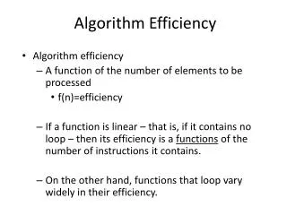
Analysis of Algoithms • An investigation of an algorithm’s efficiency with respect to two resources: • Running time (time efficiency or time complexity) • Memory space (space efficiency or space complexity)
Analysis Framework • Measuring an input’s size • Measuring Running Time • Orders of Growth (of algorithm’s efficiency function) • Worst-case, Best-case, and Average-case efficiency
Measuring Input Size • Efficiency is defined as a function of input size • Input size depends on the problem • Example 1: what is the input size for sorting n numbers? • Example 2: what is the input size for evaluating ⋯ • Example 3: what is the input size for multiplying two n×n matrices?
Units of measuring running time • Measure running time in milliseconds, seconds, etc. • Depends on which computer • Count the number of times each operation is executed • Difficult and unnecessary • Count the number of times an algorithm’s “basic operation” is executed
Measure running time in terms of # of basic operations • Basic operation: the operation that contributes the most to the total running time of an algorithm • Usually the most time consuming operation in the algorithm’s innermost loop
Theoretical Analysis of Time Efficiency • Count the number of times the algorithm’s basic operation is executed on inputs of size n: C(n) T(n) ≈ cop × C(n) Input size Ignore cop, Focus on orders of growth # of times basic op. is executed Running time Execution time for basic operation If C(n) = , how much longer it runs if the input size is doubled?
Orders of Growth • Why do we care about the order of growth of an algorithm’s efficiency function, i.e., the total number of basic operations? How fast efficiency function grows as n gets larger and larger…
Orders of Growth (contd.) • Plots of growth… • Consider only the leading term • Ignore the constant coefficients
Worst, Best, Average Cases • Efficiency depends on input size n • For some algorithms, efficiency depends on the type of input • Example: Sequential Search • Given a list of n elements and a search key k, find if k is in the list • Scan list, compare elements with k until either found a match (success), or list is exhausted (failure)
Sequential Search Algorithm ALGORITHM SequentialSearch(A[0..n-1], k) //Input: A[0..n-1] and k //Output: Index of first match or -1 if no match is //found i <- 0 whilei < n and A[i] ≠ k do i <- i+1 ifi < n returni //A[i] = k else return -1
Different cases • Worst case efficiency • Efficiency (# of times the basic op. will be executed) for the worst case input of size n • Runs longest among all possible inputs of size n • Best case efficiency • Runs fastest among all possible inputs of size n • Average case efficiency • Efficiency for a typical/random input of size n • NOT the average of worst and best cases • How do we find average case efficiency?
Average Case of Sequential Search • Two assumptions: • Probability of successful search is p (0 ≤ p ≤ 1) • Search key can be at any index with equal probability (uniform distribution) Cavg(n) = Expected # of comparisons = Expected # of comparisons for success + Expected # of comparisons if k is not in the list
Summary of Analysis Framework • Time and space efficiencies are functions of input size • Time efficiency is # of times basic operation is executed • Space efficiency is # of extra memory units consumed • Efficiencies of some algorithms depend on type of input: requiring worst, best, average case analysis • Focus is on order of growth of running time (or extra memory units) as input size goes to infinity
Asymptotic Growth Rate • 3 notations used to compare orders of growth of an algorithm’s basic operation count • O(g(n)): Set of functions that grow no faster than g(n) • Ω(g(n)): Set of functions that grow at least as fast as g(n) • Θ(g(n)): Set of functions that grow at the same rate as g(n)
O(big oh)-Notation c × g(n) t(n) Doesn’t matter n n0 t(n) є O(g(n))
O-Notation (contd.) • Definition: A function t(n) is said to be in O(g(n)), denoted t(n) є O(g(n)), if t(n) is bounded above by some positive constant multiple of g(n) for sufficiently large n. • If we can find +ve constants c and n0 such that: t(n) ≤ c × g(n) for all n ≥ n0
O-Notation (contd.) • Is 100n+5 є O(n2) ? • Is 2n+1є O(2n) ? Is 22nє O(2n) ? • Is n(n-1) є O(n2) ?
Ω(big omega)-Notation t(n) c × g(n) Doesn’t matter n n0 t(n) єΩ(g(n))
Ω-Notation (contd.) • Definition: A function t(n) is said to be in Ω(g(n)) denoted t(n) єΩ(g(n)), if t(n) is bounded below by some positive constant multiple of g(n) for all sufficiently large n. • If we can find +ve constants c and n0 such that t(n) ≥ c × g(n) for all n ≥ n0
Ω-Notation (contd.) • Is n3єΩ(n2)? • Is 100n+5 єΩ(n2) ? • Is n(n-1) єΩ(n2) ?
Θ(big theta)-Notation c1 × g(n) t(n) c2× g(n) Doesn’t matter n n0 t(n) єΘ(g(n))
Θ-Notation (contd.) • Definition: A function t(n) is said to be in Θ(g(n)) denoted t(n) єΘ(g(n)), if t(n) is bounded both above and below by some positive constant multiples of g(n) for all sufficiently large n. • If we can find +ve constants c1, c2, and n0 such that c2×g(n) ≤ t(n) ≤ c1×g(n) for all n ≥ n0
Θ-Notation (contd.) • Is n(n-1) єΘ(n2) ? • Is n2+sin(n) єΘ(n2) ? • Is an2+bn+c єΘ(n2) for a > 0? • Is (n+a)bΘ(nb) for b > 0 ?
O, Θ, and Ω (≥) Ω(g(n)): functions that grow at least as fast as g(n) (=) Θ(g(n)):functions that grow at the same rate as g(n) g(n) (≤) O(g(n)): functions that grow no faster that g(n)
Theorem • If t1(n) є O(g1(n)) and t2(n) є O(g2(n)), then t1(n) + t2(n) є O(max{g1(n),g2(n)}) • Analogous assertions are true for Ω and Θ notations. • Implication: if sorting makes no more than n2 comparisons and then binary search makes no more than log2n comparisons, then efficiency is O(max{n2, log2n}) = O(n2)
Theorem (contd.) • If t1(n) є O(g1(n)) and t2(n) є O(g2(n)), then t1(n) + t2(n) є O(max{g1(n),g2(n)}) t1(n) ≤ c1g1(n) for n ≥ n01 and t2(n) ≤ c2g2(n) for n ≥ n02 t1(n) + t2(n) ≤ c1g1(n) + c2g2(n) for n ≥ max { n01, n02 } t1(n) + t2(n) ≤ max{c1, c2}g1(n) + max{c1, c2} g2(n) for n ≥ max { n01, n02 } t1(n) + t2(n) ≤ 2max{c1, c2}max{g1(n), g2(n) }, for n ≥ max{n01, n02} c n0
Using Limits for Comparing Orders of Growth 0 implies that t(n) grows slower than g(n) • = c implies that t(n) grows at the same order as g(n) ∞ implies that t(n) grows faster than g(n) 1. First two cases (0 and c) means t(n) є O(g(n)) 2. Last two cases (c and ∞) means t(n) єΩ(g(n)) 3. The second case (c) means t(n) єΘ(g(n))
Taking Limits • L’Hôpital’s rule: if limits of both t(n) and g(n) are ∞ as n goes to ∞, • Stirling’s formula:For large n, we have n! ≈
Stirling’s Formula n! ≈ • n! = n (n-1) (n-2) … 1 • ln(n!) = • Trapezoidal rule: • Add to both sides, • Exponentiate both sides, n! ≈ C nne-nn1/2 = C … 1 2 3 4 n
Taking Limits (contd.) • Compare orders of growth of 22n and 3n • Compare orders of growth of lgn and • Compare orders of growth of n! and 2n
Summary of How to Establish Order of Growth of Basic Operation Count • Method 1: Using Limits • Method 2: Using Theorem • Method 3: Using definitions of O-, Ω-, and Θ-notations.
Analysis of Nonrecursive Algorithms ALGORITHM MaxElement(A[0..n-1]) //Determines largest element maxval <- A[0] fori <- 1 to n-1 do if A[i] > maxval maxval <- A[i] returnmaxval Input size: n Basic operation: > or <- C(n) = єΘ(n)
General Plan for Analysis of Nonrecursive algorithms • Decide on a parameter indicating an input’s size • Identify the basic operation • Does C(n) depends only on n or does it also depend on type of input? • Set up sum expressing the # of times basic operation is executed. • Find closed form for the sum or at least establish its order of growth
Analysis of Nonrecursive (contd.) ALGORITHM UniqueElements(A[0..n-1]) //Determines whether all elements are //distinct fori <- 0 to n-2 do for j <- i+1 to n-1 do if A[i] = A[j] return false return true Input size: n Basic operation: A[i] = A[j] Does C(n) depend on type of input?
UniqueElements (contd.) fori <- 0 to n-2 do for j <- i+1 to n-1 do if A[i] = A[j] return false return true Cworst(n) = Why Cworst(n) is better than saying Cworst(n)
Analysis of Nonrecursive(contd.) ALGORITHM MatrixMultiplication(A[0..n-1, 0..n-1], B[0..n-1, 0..n-1]) //Output: C = AB fori <- 0 to n-1 do for j <- 0 to n-1 do C[i, j] = 0.0 for k <- 0 to n-1 do C[i, j] = C[i, j] + A[i, k]×B[k, j] return C T(n) ≈ cmM(n)+caA(n) = cmn3+can3 = (cm+ca)n3 Input size: n Basic operation: × M(n) =
Analysis of Nonrecursive (contd.) ALGORITHM Binary(n) // Output: # of digits in binary // representation of n count <- 1 while n > 1 do count <- count+1 n <- return count Input size: n Basic operation: C(n) = ? Each iteration halves n Let m be such that 2m ≤ n < 2m+1 Take lg: m ≤ lg(n) < m+1, so m = and m+1 = +1 єΘ(lg(n))
Analysis of Nonrecursive (contd.) ALGORITHM Mystery(n) S <- 0 fori <- 1 to n do S <- S + i×i return S What does this algorithm compute? What is the basic operation? How many times is the basic operation executed? What’s its efficiency class? Can you improve it further, or Can you prove that no improvement is possible?
Analysis of Nonrecursive (contd.) What does this algorithm compute? ALGORITHM Secret(A[0..n-1]) r <- A[0] s <- A[0] fori <- 1 to n-1 do if A[i] < r r <- A[i] if A[i] > s s <- A[i] return s-r What is the basic operation? How many times is the basic operation executed? What’s its efficiency class? Can you improve it further, Or Could you prove that no improvement is possible?
Analysis of Recursive Algorithms ALGORITHM F(n) // Output: n! if n = 0 return 1 else returnn×F(n-1) Input size: n Basic operation: × M(n) = M(n-1) + 1 for n > 0 to compute F(n-1) to multiply n and F(n-1)
Analysis of Recursive (contd.) Recurrence relation M(n) = M(n-1) + 1 M(0) = 0 M(n) = M(n-1) + 1 = M(n-2)+ 1 + 1 = … … = M(n-n) + 1 + … + 1 = 0 + n = n We could compute it nonrecursively, saves function call overhead By Backward substitution n 1’s
General Plan for Recursive • Decide on input size parameter • Identify the basic operation • Does C(n) depends also on input type? • Set up a recurrence relation • Solve the recurrence or, at least establish the order of growth of its solution
Tower of Hanoi (contd.) M(n-1) M(n) = M(n-1) + 1 + M(n-1) M(1) = 1 1 M(n-1)