Algorithm Efficiency
Algorithm Efficiency. Design & Analysis of Algorithms CS315. Analysis of algorithms. Issues: Correctness Time efficiency Space efficiency Optimality Approaches: Theoretical analysis Empirical analysis. Algorithm Correctness. Correct with respect to a specification.

Algorithm Efficiency
E N D
Presentation Transcript
Algorithm Efficiency Design & Analysis of AlgorithmsCS315
Analysis of algorithms • Issues: • Correctness • Time efficiency • Space efficiency • Optimality • Approaches: • Theoretical analysis • Empirical analysis
Algorithm Correctness • Correct with respect to a specification. • Functional correctness • Refers to the input-output behavior of the algorithm (i.e., for each input it produces the correct output) • Total correctness • Requires that the algorithm terminates • Partial correctness • If an answer is returned it will be correct
Algorithm Time Efficiency • For the analysis to correspond usefully to the actual execution time, the time required to perform a step must be guaranteed to be bounded above by a constant
Algorithm Time Efficiency • Two cost models are generally used: • Uniform cost model • Also called uniform-cost measurement (and similar variations) • Assigns a constant cost to every machine operation, regardless of the size of the numbers involved • Logarithmic cost model • Also called logarithmic-cost measurement • Assigns a cost to every machine operation proportional to the number of bits involved
input size running time Number of times basic operation is executed execution time for basic operation Theoretical analysis of time efficiency Time efficiency is analyzed by determining the number of repetitions of the basic operation as a function of input size • Basic operation: the operation that contributes most towards the running time of the algorithm T(n) ≈copC(n)
Empirical analysis of time efficiency • Select a specific (typical) sample of inputs • Use physical unit of time (e.g., milliseconds) or … • Count actual number of basic operation’s executions • Analyze the empirical data
Best-case, average-case, worst-case For some algorithms efficiency depends on form of input: • Worst case: Cworst(n) – maximum over inputs of size n • Best case: Cbest(n) – minimum over inputs of size n • Average case: Cavg(n) – “average” over inputs of size n • Number of times the basic operation will be executed on typical input • NOT the average of worst and best case … Why? • Expected number of basic operations considered as a random variable under some assumption about the probability distribution of all possible inputs
Example: Sequential search • Which step would you count?
Example: Sequential search • What’s the … • Worst case • Best case • Average case
Types of formulas for basic operation’s count • Exact formula e.g., C(n) = n(n-1)/2 • Formula indicating order of growth with specific multiplicative constant e.g., C(n) ≈ 0.5 n2 • Formula indicating order of growth with unknown multiplicative constant e.g., C(n) ≈cn2
Order of growth • Most important: Order of growth within a constant multiple as n→∞ • Example: • How much faster will algorithm run on computer that is twice as fast? • How much longer does it take to solve problem of double input size?
Asymptotic order of growth A way of comparing functions that ignores constant factors and small input sizes • O(g(n)): class of functions f(n) that grow no faster than g(n) • Θ(g(n)): class of functions f(n) that grow at same rate as g(n) • Ω(g(n)): class of functions f(n) that grow at least as fast as g(n)
Establishing order of growth • f(n) is O(g(n)) IF • Order of growth of f(n) ≤ order of growth of g(n) (within constant multiple) • There exist positive constant c and non-negative integer n0 such that …f(n) ≤ c g(n) for every n ≥ n0 Examples: • 5n2 - 10n is O(n2) • 5n+20 is O(n) How do we prove this?
Properties • f(n) O(f(n)) • f(n) O(g(n)) iff g(n) (f(n)) • If f(n) O(g(n)) and g(n) O(h(n)) , then f(n) O(h(n)) • Note similarity with a ≤ b • If f1(n) O(g1(n)) and f2(n) O(g2(n)) , then f1(n) +f2(n) O(max{g1(n), g2(n)})
0 order of growth of T(n) < order of growth of g(n) c > 0 order of growth of T(n) = order of growth of g(n) ∞ order of growth of T(n) > order of growth of g(n) Using limits limT(n)/g(n) = n→∞ • Examples: • 10n vs. n2 • n(n+1)/2 vs. n2
f ´(n) g ´(n) f(n) g(n) lim n lim n = L’Hôpital’s rule and Stirling’s formula L’Hôpital’s rule: If limnf(n) = limng(n) = and the derivatives f´, g´ exist, then Stirling’s formula: n! (2n)1/2 (n/e)n Example: log n vs. n Example: 2n vs. n!
Orders of growth of some important functions • All logarithmic functions loga n belong to the same class (log n) no matter what the logarithm’s base a > 1 isWHY?
Orders of growth of some important functions • All polynomials of the same degree k belong to the same class: aknk + ak-1nk-1 + … + a0 (nk)WHY?
Orders of growth of some important functions • Exponential functions an have different orders of growth for different a’sWHY?
Orders of growth of some important functions • Order log n < order n (>0) < order an < order n! < order nnWHY?
Time efficiency of non-recursive algorithms General Plan for Analysis • Decide on parameter n indicating input size • Identify algorithm’s basic operation • Determine worst, average, and best cases for input of size n • Set up a sum for the number of times the basic operation is executed • Simplify the sum using standard formulas and rules (see Appendix A)
Useful summation formulas and rules • liu1 = 1+1+ ⋯ +1 = u -l + 1In particular, liu1 = n - 1 + 1 = n (n) • 1ini = 1+2+ ⋯ +n = n(n+1)/2 n2/2 (n2) • 1ini2 = 12+22+ ⋯ +n2 = n(n+1)(2n+1)/6 n3/3 (n3)
Useful summation formulas and rules • 0inai = 1+ a + ⋯ + an = (an+1 - 1)/(a - 1)for any a 1In particular, 0in2i = 20 + 21 + ⋯ + 2n = 2n+1- 1 (2n) • (ai±bi ) = ai± bi cai = cailiuai = limai+ m+1iuai
Example 2: Element uniqueness problem Could you rewrite this so there was only one return step?
Example 4: Gaussian elimination • In linear algebra, an algorithm for solving systems of linear equations • Can also be used to find the rank of a matrix, to calculate the determinant of a matrix, and to calculate the inverse of an invertible square matrix • Named after Carl Friedrich Gauss, but it was not invented by him
Example 4: Gaussian elimination AlgorithmGaussianElimination(A[0..n-1,0..n]) //Implements Gaussian elimination of an n-by-(n+1) matrix A for i0 to n -2 dofor ji+ 1 to n - 1 do for ki to n do A[j,k] A[j,k] -A[i,k] A[j,i] / A[i,i] Find the efficiency class and a constant factor improvement.
Example 5: Counting binary digits It cannot be investigated the way the previous examples are.
Plan for Analysis of Recursive Algorithms • Decide on a parameter indicating an input’s size. • Identify the algorithm’s basic operation. • Check whether the number of times the basic op. is executed may vary on different inputs of the same size. (If it may, the worst, average, and best cases must be investigated separately.) • Set up a recurrence relation with an appropriate initial condition expressing the number of times the basic op. is executed. • Solve the recurrence (or, at the very least, establish its solution’s order of growth) by backward substitutions or another method.
Example 1: Recursive evaluation of n! Definition: n ! = 1 2 … (n-1) n for n ≥ 1 and 0! = 1 Recursive definition of n!: F(n) = F(n-1) n for n ≥ 1 and F(0) = 1 Size: Basic operation: Recurrence relation:
Solving the recurrence for M(n) M(n) = M(n-1) + 1, M(0) = 0
Example 2: The Tower of Hanoi Puzzle Recurrence for number of moves:
Solving recurrence for number of moves M(n) = 2M(n-1) + 1, M(1) = 1
Fibonacci numbers The Fibonacci numbers: 0, 1, 1, 2, 3, 5, 8, 13, 21, … The Fibonacci recurrence: F(n) = F(n-1) + F(n-2) F(0) = 0 F(1) = 1 General 2nd order linear homogeneous recurrence with constant coefficients: aX(n) + bX(n-1) + cX(n-2) = 0
Solving aX(n) + bX(n-1) + cX(n-2) = 0 • Set up the characteristic equation (quadratic) ar2 + br + c= 0 • Solve to obtain roots r1 and r2 • General solution to the recurrence if r1 and r2 are two distinct real roots: X(n) = αr1n + βr2n if r1 =r2 = r are two equal real roots: X(n) = αrn+ βnrn • Particular solution can be found by using initial conditions
Application to the Fibonacci numbers F(n) = F(n-1) + F(n-2) or F(n) - F(n-1) - F(n-2) = 0 Characteristic equation: Roots of the characteristic equation: General solution to the recurrence: Particular solution for F(0) =0, F(1)=1:
n F(n-1) F(n) 0 1 = F(n) F(n+1) 1 1 Computing Fibonacci numbers • Definition-based recursive algorithm • Non-recursive definition-based algorithm • Explicit formula algorithm • Logarithmic algorithm based on formula: for n≥1, assuming an efficient way of computing matrix powers.