Chapter 23 Algorithm Efficiency
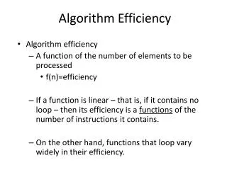
Chapter 23 Algorithm Efficiency. Objectives (1). To estimate algorithm efficiency using the Big O notation (§23.2) To understand growth rates and why constants and smaller terms can be ignored in the estimation (§23.2)

Chapter 23 Algorithm Efficiency
E N D
Presentation Transcript
Objectives (1) • To estimate algorithm efficiency using the Big O notation (§23.2) • To understand growth rates and why constants and smaller terms can be ignored in the estimation (§23.2) • To know the examples of algorithms with constant time, logarithmic time, linear time, log-linear time, quadratic time, and exponential time (§23.2) • To analyze linear search, binary search, selection sort, and insertion sort (§23.2)
Objectives (2) • To design, implement, and analyze bubble sort (§23.3) • To design, implement, and analyze merge sort (§23.4) • To design, implement, and analyze quick sort (§23.5) • To design, implement, and analyze heap sort (§23.6) • To sort large data in a file (§23.7)
Analysis of Algorithms Input Algorithm Output An algorithm is a step-by-step procedure for solving a problem in a finite amount of time
Characterizing Algorithms • Investigating the run times of algorithms and data structure operations • Focus will be on the relationship between running time of an algorithms and the size of the input
Can We Write Better Algorithms? “Better.” ―Michelangelo, when asked how he would have made his statue of Moses if he had to do it over again
Executing Time Question • Suppose two algorithms perform the same task such as search (linear search vs. binary search) and sorting (selection sort vs. insertion sort) • Which one is better? • One possible approach to answer this question is to implement these algorithms in Java and run the programs to get execution time • But there are two problems with this approach…..
Problems Measuring Execution Time • First, there are many tasks running concurrently on a computer • The execution time of a particular program is dependent on the system load • Second, the execution time is dependent on specific input • Consider linear search and binary search • If an element to be searched happens to be the first in the list, linear search will find the element quicker than binary search
Growth Rate of Running Time • Changing the hardware/ software environment • Affects running time by a constant factor • It but does not alter the growth rate
Experimental Studies • Write a program implementing an algorithm • Run the program with inputs of varying size and composition • Use a method like System.currentTimeMillis()to get an accurate measure of the actual running time • Plot the results
Limitations of Experiments • It is necessary to implement the algorithm, which may be difficult • Results may not be indicative of the running time on other inputs not included in the experiment • In order to compare two algorithms, the same hardware and software environments must be used
Theoretical Analysis • Uses a high-level description of the algorithm instead of an implementation • Characterizes running time as a function of the input size, n • Takes into account all possible inputs • Allows us to evaluate the speed of an algorithm independent of the hardware/software environment
Growth Rate (1) • It is very difficult to compare algorithms by measuring their execution time • To overcome these problems, a theoretical approach was developed to analyze algorithms independent of computers and specific input • This approach approximates the effect of a change on the size of the input
Growth Rate (2) • In this way, one can see how fast an algorithm’s execution time increases as the input size increases, so one can compare two algorithms by examining their growth rates
Execution Time (1) • The linear search algorithm compares the key with the elements in the array sequentially until the key is found or the array is exhausted • If the key is not in the array, it requires n comparisons for an array of size n • If the key is in the array, it requires n/2 comparisons on average
Execution Time (2) • The algorithm’s execution time is proportional to the size of the array • If one doubles the size of the array, one will expect the number of comparisons to double • The algorithm grows at a linear rate • The growth rate has an order of magnitude of n
Big O Notation • Computer scientists use the Big O notation to abbreviate for “order of magnitude” • ” Using this notation, the complexity of the linear search algorithm is O(n),pronounced as “order of n”
Best, Worst, and Average Cases • For the same input size, an algorithm’s execution time may vary, depending on the input • An input that results in the shortest execution time is called the best-case input and an input that results in the longest execution time is called the worst-case input • Best-caseand worst-case are not representative, but worst-case analysis is very useful • One can show that the algorithm will never be slower than the worst-case • An average-case analysis attempts to determine the average amount of time among all possible input of the same size
Worse Case • Average-case analysis is ideal, but difficult to perform, because it is hard to determine the relative probabilities and distributions of various input instances for many problems • Worst-case analysis is easier to obtain and is thus common • Analysis is generally conducted for the worst-case • Crucial to applications such as games, finance and robotics
Useful Formulas Arithmetic sum Geometric sum
Summation Notation Polynomials
Seven Functions • These functions are often used in algorithm analysis • Constant 1 • Logarithmic log n • Linear n • n-log-n n log n • Quadratic n2 • Cubic n3 • Exponential 2n
Constant Function • f (n) = c • Typically f (n) = 1 is used during algorithm analysis • A constant function is used to characterize the number of steps needed to do a basic operations • Time is not related to the input size • Adding two numbers • Assigning a value to a variable • Comparing two numbers • Retrieves an element at a given index in an array
Logarithm Function • f (n) = logbnfor some constant b • The function is defined as follows • x= logbnif and only ifbx=n • 2 is the most common base used during algorithms analysis • If one squares the input size, one only doubles the time for the algorithm of O(logn)
Basic Properties of Logarithms logb(xy) = logbx + logby logb (x/y) = logbx - logby logbxa = alogbx logba = logda/logdb b logda = a logdb log2n= log n/ log2 (converts base 10 to base 2)
Linear Function • f (n) = n • Function arises when the same basic operation is done for n elements • For example • Comparing a constant c to each element of an array of size n requires n comparisons • Reading n objects requires n operations
n-log-n Function • f (n) = n log2n • This function • Grows a little faster than the linear function, f (n) =n • Grows much slower than the quadratic n2 , f (n) = n2 • If we can improve the running time of solving some problem from a quadratic to n-log-n, we will have an algorithm that runs much faster
Quadratic Function • f (n) = n2 • This function is used in analysis since many algorithms contain nested loops • The inner loop performs n operations while the outer loop performs n operations (n * n = n2)
Quadratic Time • An algorithm with the O(n2) time complexity is called a quadratic algorithm • The quadratic algorithm grows quickly as the problem size increases • If one doubles the input size, the time for the algorithm is quadrupled • Algorithms with a nested loop are often quadratic
Nested Loops and the Quadratic Function • The quadratic function also is used in the context of nested loops where the first iteration uses one operation, the second uses two operations, the third uses three operations, and so on (for the inner loop) for (inti = 0; i < n; i++) { for (int j = 0; j < i; j++) { { System.out.print('*'); } }
Nested Loops and the Quadratic Function • The number of operations performed is • 1 + 2 + 3+ … + (n-2) + (n-1) + n = n(n+1)/2=(n2+n)/2 =n2/2+n/2 • Note: n2 >(n2+n)/2 • An algorithm characterized where the first iteration uses one operation, the second uses two operations, the third uses three operations and so on, is slightly better than an algorithm that uses n operations each time through the loop (n2)
Cubic Function • f (n) = n3 • This function is used often used in algorithm analysis
Polynomials • f (n) = ao +a1n +a2n2+… adnd • This function has degree d • Running times that are polynomials with degree d are generally better than polynomials with a larger degree • Note: the constant, linear, quadratic, and cubic functions are polynomials
Exponential Function • f (n) = bn • Most common based used in algorithm analysis is 2 • If a loops starts by performing one operation and then doubles the number of operations performed within each iteration • The number of operations performed in the nthiteration is 2n
Basic Properties of Exponentials (ab)c = abc abac = a(b+c) ab/ac = a(b-c)
Comparison of Functions • The slope of the line corresponds to the growth rate of the function
Big-Oh Inequality • Let f(n)and g(n) be non-negative functions • Then f(n)is O(g(n)) if there are positive constant c and n0 1 such that f(n)cg(n) for n n0 • This definition is referred to as the big-Ohnotation or f(n) is big-Oh of g(n) or f(n)is order of g(n)
Big-Oh and Growth Rate • The big-Oh notation gives an upper bound on the growth rate of a function • The statement “f(n) is O(g(n))” means that the growth rate of f(n)is no more than the growth rate of g(n)
Ignoring Multiplicative Constants • The linear search algorithm requires n comparisons in the worst-case and n/2 comparisons in the average-case • Using the Big O notation, both cases require O(n)time • The multiplicative constant (1/2) is normally omitted • Algorithm analysis is focused on growth rate • The multiplicative constants have little impact on growth rates • The growth rates n/2 and 100n are equivalent to n • O(n) = O(n/2) = O(100n)
Ignoring Non-Dominating Terms (1) • Consider the algorithm for finding the maximum number in an array of n elements • If n is 2, it takes one comparison to find the maximum number • If n is 3, it takes two comparisons to find the maximum number • In general, it takes n-1 times of comparisons to find maximum number in a list of nelements If the input size is small, there is no significance to estimate an algorithm’s efficiency
Ignoring Non-Dominating Terms (2) • Algorithm analysis is done for large input sizes • If is f(n) a polynomial of degree d, then f(n) is O(nd), • Drop lower-order terms • Drop constant factors • As n grows larger, the n part in the expression n-1dominates the complexity
Big-Oh Rules • Use the smallest possible class of functions • Say “2n is O(n)” instead of “2n is O(n2)” • Use the simplestexpression of the class • Say “3n + 5 is O(n)” instead of “3n + 5 is O(3n)”
Big-Oh Example (1) • 8n - 2 is O(n) • Justification • Find c and n0 such that 8n-2 cn • Pick c = 8 and n0 = 1 (there are an infinite number of solutions) 8n - 2 8n
Big-Oh Example (2) • 2n +10 is O(n) • Justification 2n + 10 cn 2n-cn -10 n(2-c) -10 n(c-2) 10 n 10/(c-2) Let c=3 and n0=10
Big-Oh Examples (3) • 5n4+3n3+2n2+4n+1 is O(n4) • Justification • 5n4+3n3+2n2+4n+1 (5+3+2+4+1) n4 =cn4 where c=15 and n0=1 • 5n2+3log(n)+2n+5 is O(n2) • Justification • 5n2+3log(n)+2n+5 (5+3+2+5) n2=cn2 where c=15 and nn0=1
Big-Oh Examples (4) • 20n3+10nlog(n)+5 is O(n3) • Justification • 20n3+10nlog(n)+5 35 n3 =cn3 where c=35 and nn0=2 • 3log(n)+2 is O(log n) • Justification • 3log(n)+2 5 log(n)where c=5 and n2
Big-Oh Examples (5) • 2n+1is O(2n) • Justification • 2n+1 = 2n *21 =2* 2n 2* 2n where c=2 and n0=1 • 2n+100log(n) is O(n) • Justification • 2n+100log(n) 102nwhere c=102 and n n0=2 • 3 log n + 5 is O(log n) • Justification • 3 log n + 5 8 log n where c = 8 and n0 = 2
Big-Oh Example (6) • n2is not O(n) • Justification n2cn n c • The above inequality cannot be satisfied since c must be a constant
Increasing Common Growth Functions Constant time Logarithmic time Linear time Log-linear time Quadratic time Cubic time Exponential time