Algorithm Efficiency and Sorting
Algorithm Efficiency and Sorting. (Walls & Mirrors - Beginning of Chapter 9). Overview. Basics of Algorithm Efficiency Efficiency of Search Algorithms Selection Sort Bubble Sort Insertion Sort. Basics of Algorithm Efficiency.

Algorithm Efficiency and Sorting
E N D
Presentation Transcript
Algorithm Efficiency and Sorting (Walls & Mirrors - Beginning of Chapter 9)
Overview • Basics of Algorithm Efficiency • Efficiency of Search Algorithms • Selection Sort • Bubble Sort • Insertion Sort
Basics of Algorithm Efficiency • We are interested in looking for significant differences in the efficiency of different methods of solution. • Since efficiency differences are either not apparent or irrelevant when the problem to be solved is small, we shall restrict our attention to efficiency differences when solving largeproblems only. • Since none of the methods we shall consider has significant space requirements, we shall focus primarily on time efficiency.
Program Efficiency • We consider the efficiency of algorithms instead of programs because of the following. • Program efficiency depends on: • How the program was implemented. Coding “tricks” may cause one algorithm to appear faster than another, but at the cost of readability and maintainability. Also, such tricks rarely cause significant differences in efficiency when solving large problems. • Speed of the computer on which a program is run. • Choice of data.
Algorithm Efficiency • To compare different methods of solution, (or algorithms), independent of the preceding factors, we shall count significant algorithmic operations and consider average and worst-case performance. • Significant algorithmic operations include: • Number of data-item comparisons, and • Number of data-item moves
5 8 13 21 34 55 . . . 610 0 1 2 3 4 5 N-1 Algorithm Efficiency: Example Problem: Search an array of N integers to find a given value. Suppose that the array looks like this: • If we are doing a sequential search, say for 610, we might have to look through all N elements of the array, comparing the desired value with each element (worst case). • If N = 1,000,000, this would require 1,000,000 comparisons (and take a while!). • However, the binary search we presented in Lecture 2 would require only lg(1000000)=20 comparisons (worst case).
Algorithm Efficiency: Why Care? • Suppose that you have an algorithm that requires 2N operations to process N data items. • For N = 100, 2N 1030. • A computer with a 100 MHz internal clock operates at 108 cycles per second. In the bestcase, let’s say that each algorithmic operation can be done in one of these cycles. • Now, 1030 operations on this computer will require 1030/108 = 1022 seconds. • Since there are 31,536,000 seconds in a year, processing 100 data items will require 1022 / (3.1536*107) > 1014 = 100,000 BILLION YEARS!
Growth Rate Comparison (Cont’d.) • If we have the opportunity to choose either an algorithm that takes 10*N time units to run or an algorithm that takes 0.1*N2 time units to run, it would be better to choose the 10*N solution, since this would take less time for any N > 100. • For small values of N, we probably don’t care which solution is chosen.
Order of an Algorithm • Definition: Algorithm A is order f(N), denoted O( f(N) ), if there is some constant C, such that for all but a finite number of exceptions, A can solve a problem of size N in time C * f(N). • O( f(N) ) is called “big O notation” to distinguish it from o( f(N) ), “little o notation,” which defines a stricter bound on A’s time requirements. (“Little o notation” is beyond the scope of this course.) • f(N) is called the growth-rate function for A.
Properties of Growth-Rate Functions 1) You can ignore low-order terms. O( N3 + 4 N2 + 3 N) = O( N3 ) The reason for this is that, for any growth-rate function, f(N), we are interested in the growth rate of f(N),not the value of f for any particular value of N. For largeN, the growth rate of N 3 is the same as the growth rate of N 3 + 4 N 2 + 3 N. 2) You can ignore a multiplicative constants. O( 5 N3 ) = O( N3 ) These constants just change the value of C in the definition of O( f(N) ). Namely, algorithm A takes time C * f(N). 3) You can combine growth-rate functions: O( f(N) ) + O( g(N) ) = O( f(N) + g(N) ) If O(f(N)) = O(g(N)) = O(N), then O( f(N) + g(N) ) = O(N)
Efficiency of Sequential Search Problem: Search for a desired item in a list of N items. • In the best case, the desired item is the first one you examine. This makes the best case O(1). • In the worst case, you have to examine all N items. This makes the worst caseO(N). • In the average case, we have to examine N/2 items. This makes the average caseO(N/2) = O(N).
Efficiency of Binary Search Problem: Search for a desired item in a sorted list of N items. • First, we compare the middle item with the desired item. If they match, we are done. If they don’t match, then we select half of the list and examine the middle of it. We continue in this manner until either the item is found or we are left with a subset of the list with only one non-matching item. • If N = 2k, for some k, then in the worst case we can divide the list of N things k times (since N / 2k = 1). • Since N = 2k, k = log2 N. • Therefore, binary search has a worst case of O( log2N ).
Efficiency of Binary Search (Cont’d.) • What if N is not a power of 2 ? • Binary search still requires at mostk subdivisions, where k is the smallest integer such that 2 k-1 < N < 2 k • It follows that k – 1 < log2 N < k k < 1 + log2 N < k + 1 k = 1 + log2 N = 1 + log2 N (rounded down) • Therefore, binary search has a worst case of O( log2N ), even if N is not a power of 2. • Further analysis shows that the average case for binary search is also O( log2N ).
Selection Sort: Basic Idea 1) Find the largest element. 2) Swap the last element with the largest. 3) Repeat steps 1 and 2 for a list with one fewer elements. 4) Continue until you have produced a sublist containing 2 elements and placed them in the correct order.
29 10 14 13 37 0 1 2 3 4 29 10 14 37 13 0 1 2 3 4 Selection Sort: Example Problem: Sort the following array from smallest to largest. • The largest element is in position 3. So, we swap this with the last element (position 4), yielding • The element now in position 4 is in its final position and will not move again throughout the remainder of the algorithm.
29 10 14 13 37 0 1 2 3 4 13 10 14 29 37 0 1 2 3 4 Selection Sort: Example (Cont’d.) • Of the elements in positions 0 through 3, the largest is in position 0. So, we swap this with the element in position 3, yielding • The element now in position 3 is in its final position and will not move again throughout the remainder of the algorithm.
13 10 14 29 37 0 1 2 3 4 13 10 14 29 37 0 1 2 3 4 Selection Sort: Example (Cont’d.) • Of the elements in positions 0 through 2, the largest is in position 2. So, we swap this with itself, yielding • The element now in position 2 is in its final position and will not move again throughout the remainder of the algorithm.
13 10 14 29 37 10 13 14 29 37 0 1 2 3 4 0 1 2 3 4 Selection Sort: Example (Cont’d.) • Of the elements in positions 0 through 1, the largest is in position 0. So, we swap this with the element in position 1, yielding • The entire list is sorted once we place the two remaining elements (positions 0 and 1) in sorted order.
Selection Sort: C++ Implementation void selectionSort( DataType a[ ], int n ) { for( int last = n – 1; last >= 1; last– – ) { // set imax to the index of the largest element in a[0 . . last] int imax = 0; for( int i = 1; i <= last; i++ ) if( a[i] > a[ imax ] ) imax = i; // swap a[imax] with a[last] DataType temp = a[last]; a[last] = a[imax]; a[imax] = temp; } }
Selection Sort: C++ Implementation void selectionSort( DataType a[ ], int n ) { for( int last = n – 1; last >= 1; last– – ) { // set imax to the index of the largest element in a[0 . . last] int imax = 0; for( int i = 1; i <= last; i++ ) if( a[i] > a[ imax ] ) imax = i; // swap a[imax] with a[last] DataType temp = a[last]; a[last] = a[imax]; a[imax] = temp; // invariant: a[last]..a[n-1] are the largest elements in sorted order } }
Selection Sort: Efficiency • The loop that finds the largest element in a[0 . . last] iterates n – 1 times on the 1st pass n – 2 times on the 2nd pass n – 3 times on the 3rd pass . . . 1 time on the last pass • One comparison of data items ( a[i] > a[ imax ] ) is made each time this loop is executed. • Therefore, the total number of data-item comparisons is: (n – 1) + (n – 2) + . . . + 1 = n * (n – 1) / 2
Selection Sort: Efficiency (Cont’d.) • a[imax] is swapped with a[last] n – 1 times. • Each swap involves 3 data-item moves. • It follows that the total number of data-item operations (comparisons and moves) is given by [ n * (n – 1) / 2 ] + [ 3 * (n – 1) ] = (1/2) * n2 + (5/2) * n – 3 • Therefore, the running time of Selection sort is O( n2 ). • According to this analysis, the running time of Selection sort is independent of the order of the input data. Consequently, it represents the best, worst, and average cases.
Selection Sort: Efficiency Caveat • Although the preceding analysis is adequate for establishing the worst-case growth rate for Selection sort, a more careful analysis shows that, in fact, the average running time is dependent on the data to be sorted. • Consider the inner loop for( int i = 1; i <= last; i++ ) if( a[i] > a[ imax ] ) imax = i; • Since imax = i is executed only when a[i] > a[imax], this assignment isdependent on the order of the data in a[0 . . n]. • Analysis that takes this into account can be found in Knuth, Donald E., The Art of Computer Programming, vol. 3, Addison-Wesley, Reading, Ma., 1973.
Bubble Sort: Basic Idea 1) Compare the first two elements. If they are in the correct order, leave them alone. Otherwise, swap them. 2) Repeat step 1 for the 2nd and 3rd elements, the 3rd and 4th elements, and so on, until the last two elements have been compared and swapped, if necessary. (When step 2 is done, the largest element will be at the end of the list.) 3) Repeat steps 1 and 2 for a list with one fewer elements. 4) Continue until you have produced a sublist containing 2 elements and placed them in the correct order.
29 10 14 37 13 10 29 14 37 13 0 1 2 3 4 0 1 2 3 4 Bubble Sort: Example Problem: Sort the following array from smallest to largest. • The elements in positions 0 and 1 are out of order, so we swap them, yielding • The elements in positions 1 and 2 are out of order, so we swap them, yielding
10 14 29 37 13 10 14 29 13 37 0 1 2 3 4 0 1 2 3 4 Bubble Sort: Example (Cont’d.) • The elements in positions 2 and 3 are in order, so we leave them alone. • The elements in positions 3 and 4 are out of order, so we swap them, yielding • The element now in position 4 is in its final position and will not move again throughout the remainder of the algorithm.
10 10 14 14 13 29 13 29 37 37 0 0 1 1 2 2 3 3 4 4 Bubble Sort: Example (Cont’d.) • The elements in positions 0 and 1 are in order, so we leave them alone. • The elements in positions 1 and 2 are in order, so we leave them alone. • The elements in positions 2 and 3 are out of order, so we swap them, yielding
10 10 13 14 14 13 29 29 37 37 0 0 1 1 2 2 3 3 4 4 Bubble Sort: Example (Cont’d.) • The element now in position 3 is in its final position and will not move again throughout the remainder of the algorithm. • The elements in positions 0 and 1 are in order, so we leave them alone. • The elements in positions 1 and 2 are out of order, so we swap them, yielding
10 13 14 29 37 0 1 2 3 4 10 13 14 29 37 0 1 2 3 4 Bubble Sort: Example (Cont’d.) • The element now in position 2 is in its final position and will not move again throughout the remainder of the algorithm. • The elements in positions 0 and 1 are in order, so we leave them alone. • The entire list is sorted once the last two elements (positions 0 and 1) are in sorted order.
Bubble Sort: Efficiency Improvement • If we can make a pass through the entire list without swapping any elements, then the list is in sorted order and the algorithm can be terminated early. • We take advantage of this fact in the following implementation.
Bubble Sort: C++ Implementation void bubbleSort( DataType a[ ], int n ) { bool sorted = false; for( int pass = 1; pass < n && !sorted; pass++ ) { sorted = true; for( int i = 0; i < n – pass; i++ ) { int inext = i + 1; if( a[i] > a[ inext ] ) { DataType temp = a[inext]; a[inext] = a[i]; a[i] = temp; sorted = false; } } } }
Bubble Sort: Efficiency • At most n – 1 passes through a[0 . . n – 1] are required. • For each pass, the inner loop executes as follows: n – 1 times on the 1st pass n – 2 times on the 2nd pass . . . 1 time on the last pass • One data-item comparison and at most one data-item exchange is required each time this loop is executed. • Therefore, in the worst case, Bubble sort will require (n – 1) + (n – 2) + . . . + 1 = n * (n – 1) / 2 comparisons and the samenumber of exchanges.
Bubble Sort: Efficiency (Cont’d.) • Since each exchange involves 3 data-item moves, it follows that the total number of data-item operations (comparisons and moves) is given by [ n * (n – 1) / 2 ] + [ 3 * n * (n – 1) / 2 ] = 2 * n2 – 2 * n • Therefore, Bubble sort has a worst-case running time of O( n2 ). • In the best case, when the list of data items is already in sorted order, Bubble sort requires n – 1 comparisons and no exchanges. In this case, Bubble sort is O( n ). • According to the analysis done by Knuth, Bubble sort’s average running time is also O( n2 ), but approximately 2.3 times the average running time of Selection sort.
Insertion Sort: Basic Idea Insertion sort is like arranging a hand of cards. As each card is dealt, that card is inserted into its proper place among the other cards in the hand so that all the cards remain in the desired order. In other words . . .
Insertion Sort: Basic Idea (Cont’d.) Let a[0 .. n – 1] denote the list to be sorted. 1) Store a[1] in local variable, value. If a[0] > value, copy it into a[1]. Now, copy value into a[0] so that a[0 .. 1] is in sorted order. 2) Store a[2] in local variable, value. If a[1] > value, copy it into a[2]. If a[0] > value, copy it into a[1]. Finally, copy value into the proper position so that a[0 .. 2] is in sorted order. 2) Store a[3] in local variable, value. If a[2] > value, copy it into a[3]. If a[1] > value, copy it into a[2]. If a[0] > value, copy it into a[1]. Finally, copy value into the proper position so that a[0 .. 3] is in sorted order. 3) Continue in this manner until a[0 .. n – 1] is in sorted order.
a[0 .. 4]: 10 value 29 10 14 37 13 0 1 2 3 4 29 29 14 37 13 a[0 .. 4]: 0 1 2 3 4 Insertion Sort: Example Problem: Sort the following array from smallest to largest. • Copy a[1] into value. Since a[0] > value, copy a[0] into a[1], yielding
10 10 value value 10 29 14 37 13 a[0 .. 4]: 29 29 14 37 13 a[0 .. 4]: 0 1 2 3 4 0 1 2 3 4 Insertion Sort: Example (Cont’d.) • Since we have reached the front of the array, copy value into a[0]. a[0..1] is now in sorted order.
10 14 value value 10 10 29 29 29 14 37 37 13 13 a[0 .. 4]: a[0 .. 4]: 0 0 1 1 2 2 3 3 4 4 Insertion Sort: Example (Cont’d.) • Copy a[2] into value. Since a[1] > value, copy a[1] into a[2], yielding
14 14 value value 10 29 29 37 13 a[0 .. 4]: 0 1 2 3 4 10 14 29 37 13 a[0 .. 4]: 0 1 2 3 4 Insertion Sort: Example (Cont’d.) • Since a[0] value, no more elements need to be examined. We have found that value needs to be copied into a[1] in order to put a[0..2] in sorted order. This results in
14 37 value value 10 10 14 14 29 29 37 37 13 13 a[0 .. 4]: a[0 .. 4]: 0 0 1 1 2 2 3 3 4 4 Insertion Sort: Example (Cont’d.) • Copy a[3] into value. Since a[2] value, no more elements need to be examined. We have found that value needs to remain in a[3] in order to put a[0..3] in sorted order. This results in
37 13 value value 10 10 14 14 29 29 37 37 37 13 a[0 .. 4]: a[0 .. 4]: 0 0 1 1 2 2 3 3 4 4 Insertion Sort: Example (Cont’d.) • Copy a[4] into value. Since a[3] > value, copy a[3] into a[4], yielding
13 13 value value 10 10 14 14 29 29 37 29 37 37 a[0 .. 4]: a[0 .. 4]: 0 0 1 1 2 2 3 3 4 4 Insertion Sort: Example (Cont’d.) • Since a[2] > value, copy a[2] into a[3], yielding
13 13 value value 10 10 14 14 29 14 29 29 37 37 a[0 .. 4]: a[0 .. 4]: 0 0 1 1 2 2 3 3 4 4 Insertion Sort: Example (Cont’d.) • Since a[1] > value, copy a[1] into a[2], yielding
13 13 value value 10 14 14 29 37 a[0 .. 4]: 10 13 14 29 37 a[0 .. 4]: 0 1 2 3 4 0 1 2 3 4 Insertion Sort: Example (Cont’d.) • Since a[0] value, no more elements need to be examined. We have found that value needs to be copied into a[1] in order to put a[0..4] in sorted order. This results in
Insertion Sort: C++ Implementation void insertionSort( DataType a[ ], int n ) { for( int unsorted = 1; unsorted < n; unsorted++ ) { int index = unsorted; DataType value = a[index]; for( ; index > 0 && a[index – 1] > value; index– – ) a[index] = a[index – 1]; a[index] = value; } }
Insertion Sort: Efficiency • At most n – 1 passes through a[0 . . n – 1] are required. • For each pass, the inner loop executes at most: 1 time on the 1st pass 2 times on the 2nd pass . . . n – 1 times on the last pass • One data-item comparison and at most one data-item move (not exchange) is required each time this loop is executed. • Therefore, in the worst case, the inner loop will require (n – 1) + (n – 2) + . . . + 1 = n * (n – 1) / 2 data-item comparisons and the samenumber of moves.
Insertion Sort: Efficiency • The outer loop moves data items twice per iteration, or 2 * (n – 1) times. • Adding it all up, we find that, in the worst case, the total number of data-item operations is given by 2 * [ n * (n – 1) / 2 ] + [ 2 * (n – 1) ] = n2 + n – 2 • Therefore, Insertion sort has a worst-case running time of O( n2 ). • In the best case, when the list of data items is already in sorted order, Insertion sort requires n – 1 comparisons and 2 * (n – 1) moves. In this case, Insertion sort is O( n ). • According to the analysis done by Knuth, Insertion sort’s average running time is also O( n2 ), but approximately 0.9 times the average running time of Selection sort and 0.4 times the average running time of Bubble sort.

