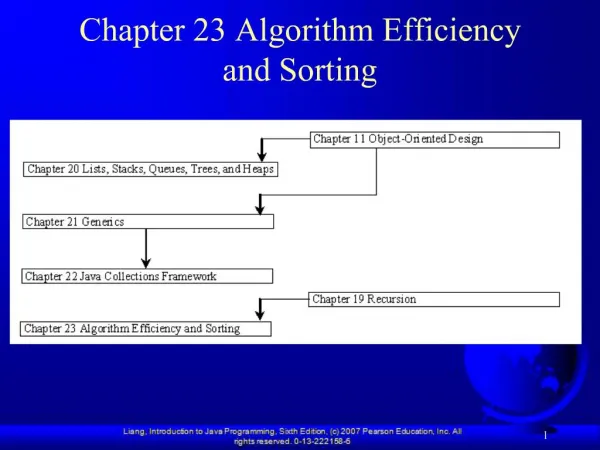
Chapter 23 Algorithm Efficiency and Sorting

1. 1 Chapter 23 Algorithm Efficiency and Sorting

2. 2 Objectives To estimate algorithm efficiency using the Big O notation (§23.2). To understand growth rates and why constants and smaller terms can be ignored in the estimation (§23.2). To know the examples of algorithms with constant time, logarithmic time, linear time, log-linear time, quadratic time, and exponential time (§23.2). To analyze linear search, binary search, selection sort, and insertion sort (§23.2). To design, implement, and analyze bubble sort (§23.3). To design, implement, and analyze merge sort (§23.4). To design, implement, and analyze quick sort (§23.5). To design, implement, and analyze heap sort (§23.6). To sort large data in a file (§23.7).

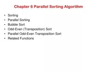
3. 3 why study sorting? Sorting is a classic subject in computer science. There are three reasons for studying sorting algorithms. First, sorting algorithms illustrate many creative approaches to problem solving and these approaches can be applied to solve other problems. Second, sorting algorithms are good for practicing fundamental programming techniques using selection statements, loops, methods, and arrays. Third, sorting algorithms are excellent examples to demonstrate algorithm performance.

4. 4 what data to sort? The data to be sorted might be integers, doubles, characters, or objects. §6.8, “Sorting Arrays,” presented selection sort and insertion sort for numeric values. The selection sort algorithm was extended to sort an array of objects in §10.5.6, “Example: Sorting an Array of Objects.” The Java API contains several overloaded sort methods for sorting primitive type values and objects in the java.util.Arrays and java.util.Collections class. For simplicity, this section assumes:

5. 5 Executing Time Suppose two algorithms perform the same task such as search (linear search vs. binary search) and sorting (selection sort vs. insertion sort). Which one is better? One possible approach to answer this question is to implement these algorithms in Java and run the programs to get execution time. But there are two problems for this approach: First, there are many tasks running concurrently on a computer. The execution time of a particular program is dependent on the system load. Second, the execution time is dependent on specific input. Consider linear search and binary search for example. If an element to be searched happens to be the first in the list, linear search will find the element quicker than binary search.

6. 6 Growth Rate It is very difficult to compare algorithms by measuring their execution time. To overcome these problems, a theoretical approach was developed to analyze algorithms independent of computers and specific input. This approach approximates the effect of a change on the size of the input. In this way, you can see how fast an algorithm’s execution time increases as the input size increases, so you can compare two algorithms by examining their growth rates.

7. 7 Big O Notation Consider linear search. The linear search algorithm compares the key with the elements in the array sequentially until the key is found or the array is exhausted. If the key is not in the array, it requires n comparisons for an array of size n. If the key is in the array, it requires n/2 comparisons on average. The algorithm’s execution time is proportional to the size of the array. If you double the size of the array, you will expect the number of comparisons to double. The algorithm grows at a linear rate. The growth rate has an order of magnitude of n. Computer scientists use the Big O notation to abbreviate for “order of magnitude.” Using this notation, the complexity of the linear search algorithm is O(n), pronounced as “order of n.”

8. 8 Best, Worst, and Average Cases For the same input size, an algorithm’s execution time may vary, depending on the input. An input that results in the shortest execution time is called the best-case input and an input that results in the longest execution time is called the worst-case input. Best-case and worst-case are not representative, but worst-case analysis is very useful. You can show that the algorithm will never be slower than the worst-case. An average-case analysis attempts to determine the average amount of time among all possible input of the same size. Average-case analysis is ideal, but difficult to perform, because it is hard to determine the relative probabilities and distributions of various input instances for many problems. Worst-case analysis is easier to obtain and is thus common. So, the analysis is generally conducted for the worst-case.

9. 9 Ignoring Multiplicative Constants The linear search algorithm requires n comparisons in the worst-case and n/2 comparisons in the average-case. Using the Big O notation, both cases require O(n) time. The multiplicative constant (1/2) can be omitted. Algorithm analysis is focused on growth rate. The multiplicative constants have no impact on growth rates. The growth rate for n/2 or 100n is the same as n, i.e., O(n) = O(n/2) = O(100n).

10. 10 Ignoring Non-Dominating Terms Consider the algorithm for finding the maximum number in an array of n elements. If n is 2, it takes one comparison to find the maximum number. If n is 3, it takes two comparisons to find the maximum number. In general, it takes n-1 times of comparisons to find maximum number in a list of n elements. Algorithm analysis is for large input size. If the input size is small, there is no significance to estimate an algorithm’s efficiency. As n grows larger, the n part in the expression n-1 dominates the complexity. The Big O notation allows you to ignore the non-dominating part (e.g., -1 in the expression n-1) and highlight the important part (e.g., n in the expression n-1). So, the complexity of this algorithm is O(n).

11. 11 Constant Time The Big O(n) notation estimates the execution time of an algorithm in relation to the input size. If the time is not related to the input size, the algorithm is said to take constant time with the notation O(1). For example, a method that retrieves an element at a given index in an array takes constant time, because it does not grow as the size of the array increases.

12. 12 Examples: Determining Big-O Repetition Sequence Selection Logarithm

13. 13 Repetition: Simple Loops for (i = 1; i <= n; i++) { k = k + 5; }

14. 14 Repetition: Nested Loops for (i = 1; i <= n; i++) { for (j = 1; j <= n; j++) { k = k + i + j; } }

15. 15 Repetition: Nested Loops for (i = 1; i <= n; i++) { for (j = 1; j <= i; j++) { k = k + i + j; } }

16. 16 Repetition: Nested Loops for (i = 1; i <= n; i++) { for (j = 1; j <= 20; j++) { k = k + i + j; } }

17. 17 Sequence for (i = 1; i <= n; i++) { for (j = 1; j <= 20; j++) { k = k + i + j; } }

18. 18 Selection if (list.contains(e)) { System.out.println(e); } else for (Object t: list) { System.out.println(t); }

19. 19 Logarithm: Analyzing Binary Search The binary search algorithm presented in Listing 6.7, BinarySearch.java, searches a key in a sorted array. Each iteration in the algorithm contains a fixed number of operations, denoted by c. Let T(n) denote the time complexity for a binary search on a list of n elements. Without loss of generality, assume n is a power of 2 and k=logn. Since binary search eliminates half of the input after two comparisons,

20. 20 Logarithmic Time Ignoring constants and smaller terms, the complexity of the binary search algorithm is O(logn). An algorithm with the time complexity is called a logarithmic algorithm O(logn). The base of the log is 2, but the base does not affect a logarithmic growth rate, so it can be omitted. The logarithmic algorithm grows slowly as the problem size increases. If you square the input size, you only double the time for the algorithm.

21. 21 Analyzing Selection Sort The selection sort algorithm presented in Listing 6.8, SelectionSort.java, finds the largest number in the list and places it last. It then finds the largest number remaining and places it next to last, and so on until the list contains only a single number. The number of comparisons is n-1 for the first iteration, n-2 for the second iteration, and so on. Let T(n) denote the complexity for selection sort and c denote the total number of other operations such as assignments and additional comparisons in each iteration. So,

22. 22 Quadratic Time An algorithm with the O(n2) time complexity is called a quadratic algorithm. The quadratic algorithm grows quickly as the problem size increases. If you double the input size, the time for the algorithm is quadrupled. Algorithms with two nested loops are often quadratic.

23. 23 Analyzing Insertion Sort The insertion sort algorithm presented in Listing 6.9, InsertionSort.java, sorts a list of values by repeatedly inserting a new element into a sorted partial array until the whole array is sorted. At the kth iteration, to insert an element to a array of size k, it may take k comparisons to find the insertion position, and k moves to insert the element. Let T(n) denote the complexity for insertion sort and c denote the total number of other operations such as assignments and additional comparisons in each iteration. So,

24. 24 Analyzing Towers of Hanoi The Towers of Hanoi problem presented in Listing 19.7, TowersOfHanoi.java, moves n disks from tower A to tower B with the assistance of tower C recursively as follows: Move the first n – 1 disks from A to C with the assistance of tower B. Move disk n from A to B. Move n - 1 disks from C to B with the assistance of tower A. Let T(n) denote the complexity for the algorithm that moves disks and c denote the constant time to move one disk, i.e., T(1) is c. So,

25. 25 Comparing Common Growth Functions Constant time

26. 26 Bubble Sort Bubble sort time: O(n2)

27. 27 Merge Sort

28. 28 Merge Sort Time Let T(n) denote the time required for sorting an array of n elements using merge sort. Without loss of generality, assume n is a power of 2. The merge sort algorithm splits the array into two subarrays, sorts the subarrays using the same algorithm recursively, and then merges the subarrays. So,

29. 29 Merge Sort Time The first T(n/2) is the time for sorting the first half of the array and the second T(n/2) is the time for sorting the second half. To merge two subarrays, it takes at most n-1 comparisons to compare the elements from the two subarrays and n moves to move elements to the temporary array. So, the total time is 2n-1. Therefore,

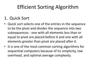
30. 30 Quick Sort Quick sort, developed by C. A. R. Hoare (1962), works as follows: The algorithm selects an element, called the pivot, in the array. Divide the array into two parts such that all the elements in the first part are less than or equal to the pivot and all the elements in the second part are greater than the pivot. Recursively apply the quick sort algorithm to the first part and then the second part.

31. 31 Quick Sort

32. 32 Partition

33. 33 Quick Sort Time To partition an array of n elements, it takes n comparisons and n moves in the worst case. So, the time required for partition is O(n).

34. 34 Worst-Case Time

35. 35 Best-Case Time

36. 36 Average-Case Time

37. 37 Heap Sort Heap sort uses a binary heap to sort an array.

38. 38 Heap Sort

39. 39 Creating an Initial Heap

40. 40 Heap Sort Time

41. 41 External Sort All the sort algorithms discussed in the preceding sections assume that all data to be sorted is available at one time in internal memory such as an array. To sort data stored in an external file, you may first bring data to the memory, then sort it internally. However, if the file is too large, all data in the file cannot be brought to memory at one time.

42. 42 Phase I Repeatedly bring data from the file to an array, sort the array using an internal sorting algorithm, and output the data from the array to a temporary file.

43. 43 Phase II Merge a pair of sorted segments (e.g., S1 with S2, S3 with S4, ..., and so on) into a larger sorted segment and save the new segment into a new temporary file. Continue the same process until one sorted segment results.

44. 44 Implementing Phase II Each merge step merges two sorted segments to form a new segment. The new segment doubles the number elements. So the number of segments is reduced by half after each merge step. A segment is too large to be brought to an array in memory. To implement a merge step, copy half number of segments from file f1.dat to a temporary file f2.dat. Then merge the first remaining segment in f1.dat with the first segment in f2.dat into a temporary file named f3.dat.

45. 45 Implementing Phase II