Chapter 23 Sorting
Chapter 23 Sorting. CS1: Java Programming Colorado State University Original slides by Daniel Liang Modified slides by Chris Wilcox. Objectives. To study and analyze time complexity of various sorting algorithms (§§23.2–23.7). To design, implement, and analyze insertion sort (§23.2).

Chapter 23 Sorting
E N D
Presentation Transcript
Chapter 23 Sorting CS1: Java Programming Colorado State University Original slides by Daniel Liang Modified slides by Chris Wilcox
Objectives • To study and analyze time complexity of various sorting algorithms (§§23.2–23.7). • To design, implement, and analyze insertion sort (§23.2). • To design, implement, and analyze bubble sort (§23.3). • To design, implement, and analyze merge sort (§23.4).
Why study sorting? Sorting is a classic subject in computer science. There are three reasons for studying sorting algorithms. • First, sorting algorithms illustrate many creative approaches to problem solving and these approaches can be applied to solve other problems. • Second, sorting algorithms are good for practicing fundamental programming techniques using selection statements, loops, methods, and arrays. • Third, sorting algorithms are excellent examples to demonstrate algorithm performance.
What data to sort? The data to be sorted might be integers, doubles, characters, or objects. §7.8, “Sorting Arrays,” presented selection sort and insertion sort for numeric values. The selection sort algorithm was extended to sort an array of objects in §11.5.7, “Example: Sorting an Array of Objects.” The Java API contains several overloaded sort methods for sorting primitive type values and objects in the java.util.Arrays and java.util.Collections class. For simplicity, this section assumes: • data to be sorted are integers, • data are sorted in ascending order, and • data are stored in an array. The programs can be easily modified to sort other types of data, to sort in descending order, or to sort data in an ArrayList or a LinkedList.
Insertion Sort The insertion sort algorithm sorts a list of values by repeatedly inserting an unsorted element into a sorted sublist until the whole list is sorted. int[] myList = {2, 9, 5, 4, 8, 1, 6}; // Unsorted
animation Insertion Sort Animation http://www.cs.armstrong.edu/liang/animation/web/InsertionSort.html
animation Insertion Sort int[] myList = {2, 9, 5, 4, 8, 1, 6}; // Unsorted
How to Insert? The insertion sort algorithm sorts a list of values by repeatedly inserting an unsorted element into a sorted sublist until the whole list is sorted.
From Idea to Solution for (int i = 1; i < list.length; i++) { insert list[i] into a sorted sublist list[0..i-1] so that list[0..i] is sorted } list[0] list[0] list[1] list[0] list[1] list[2] list[0] list[1] list[2] list[3] list[0] list[1] list[2] list[3] ...
From Idea to Solution for (int i = 1; i < list.length; i++) { insert list[i] into a sorted sublist list[0..i-1] so that list[0..i] is sorted } Expand double currentElement = list[i]; int k; for (k = i - 1; k >= 0 && list[k] > currentElement; k--) { list[k + 1] = list[k]; } // Insert the current element into list[k + 1] list[k + 1] = currentElement; Run InsertSort
Bubble Sort Bubble sort time: O(n2) Run BubbleSort
Bubble Sort Animation http://www.cs.armstrong.edu/liang/animation/web/BubbleSort.html
Merge Sort Run MergeSort
Merge Sort mergeSort(list): firstHalf = mergeSort(firstHalf); secondHalf = mergeSort(secondHalf); list = merge(firstHalf, secondHalf);
Merge Two Sorted Lists Animation for Merging Two Sorted Lists
Merge Sort Time Let T(n) denote the time required for sorting an array of n elements using merge sort. Without loss of generality, assume n is a power of 2. The merge sort algorithm splits the array into two subarrays, sorts the subarrays using the same algorithm recursively, and then merges the subarrays. So,
Merge Sort Time The first T(n/2) is the time for sorting the first half of the array and the second T(n/2) is the time for sorting the second half. To merge two subarrays, it takes at most n-1 comparisons to compare the elements from the two subarrays and n moves to move elements to the temporary array. So, the total time is 2n-1. Therefore,
Quick Sort Quick sort, developed by C. A. R. Hoare (1962), works as follows: The algorithm selects an element, called the pivot, in the array. Divide the array into two parts such that all the elements in the first part are less than or equal to the pivot and all the elements in the second part are greater than the pivot. Recursively apply the quick sort algorithm to the first part and then the second part.
Partition Animation for partition Run QuickSort
Quick Sort Time To partition an array of n elements, it takes n-1 comparisons and n moves in the worst case. So, the time required for partition is O(n).
Worst-Case Time In the worst case, each time the pivot divides the array into one big subarray with the other empty. The size of the big subarray is one less than the one before divided. The algorithm requires time:
Best-Case Time In the best case, each time the pivot divides the array into two parts of about the same size. Let T(n) denote the time required for sorting an array of elements using quick sort. So,
Average-Case Time On the average, each time the pivot will not divide the array into two parts of the same size nor one empty part. Statistically, the sizes of the two parts are very close. So the average time is O(nlogn). The exact average-case analysis is beyond the scope of this book.
Computational Complexity(Big O) • T(n)=O(1) // constant time • T(n)=O(log n) // logarithmic • T(n)=O(n) // linear • T(n)=O(nlog n) // linearithmic • T(n)=O(n2) // quadratic • T(n)=O(n3) // cubic
Complexity Examples http://bigocheatsheet.com/
Complexity Examples http://bigocheatsheet.com/