Download
1 / 36
390 likes | 662 Vues
Modeling the Upper Atmosphere and Ionosphere with TIMEGCM Geoff Crowley. Atmospheric & Space Technology Research Associates (ASTRA) www.astraspace.net. TIMEGCM: Thermosphere-Ionosphere-Mesosphere-Electrodynamics-General Circulation Model. ASPEN: A dvanced SP ace EN vironment Model.

E N D
Modeling the Upper Atmosphere and Ionosphere with TIMEGCM Geoff Crowley Atmospheric & Space Technology Research Associates (ASTRA) www.astraspace.net TIMEGCM: Thermosphere-Ionosphere-Mesosphere-Electrodynamics-General Circulation Model ASPEN: Advanced SPace ENvironment Model
Simulating Mars and Earth Temperatures, Chemistry & Winds
So it’s Easy …….. Right? Think I’ll develop another GCM this afternoon
Tides Temperature Gravity Waves Winds E-fields Composition Electron Density Simplified Physics of Upper Atmosphere Joule Heating Particle Heating Solar EUV Chemical Heating Boundary Conds Diffusion Coeffs Chemistry Solar EUV
Important Inputs to the Thermosphere – Ionosphere System Solar EUV Input OUTPUT High Latitude Inputs E-fields Particles Neutral density Composition Temperature Wind Electron density Dynamo E-fields Coupled Thermosphere –Ionosphere-Electrodynamics Tides and Gravity Waves
MODEL - QUIET - 12UT Neutral Temperature 12 UT MODEL - %DIFFERENCE (Storm – Quiet) MODEL - STORM - 12UT
MODEL - QUIET - 12UT Meridional Wind 12 UT MODEL - %DIFFERENCE (Storm – Quiet) MODEL - STORM - 12UT
Most Realistic High Latitude Inputs Data Inputs: 180 magnetometers 3 DMSP satellites X SuperDARNs
325 (11/21) 324 (11/20) 323 (11/19) 322 (11/18) 325 (11/21) 324 (11/20) 323 (11/19) 322 (11/18) Time runs right to left 325 (11/21) 324 (11/20) 322 (11/18) 323 (11/19) 325 (11/21) 324 (11/20) 323 (11/19) 322 (11/18) 325 (11/21) 324 (11/20) 323 (11/19) 322 (11/18) TIMEGCM+AMIE
Vertical Coordinate System If Zp is the pressure level (usually ranging from –17 to +5), and Po is the base pressure P = Po exp (-Zp) (ASPEN has 88 pressure levels; 30 to 600 km) Density is r = Po exp (-Zp) Mbar / (Kb T), where Kb is the Boltzman constant (gas constant / Avogadro number). Units depend on the choice of Po and Kb. If Kb = 1.38e-16 erg/K then density is in g/cm3. Horizontal Coordinates -87.5S (5) +87.5N latitude ; -180E (5) +180E longitude (72*36 grid points)
Molecular conduction radiation advection adiab. heating Many terms Energy equation The leap-frog method is employed with vertical thermal conductivity treated implicitly to second order accuracy. This leads to a tridiagonal scheme requiring boundary conditions at the top and bottom of the domain as implied by the differential equation. Advection is treated implicitly to fourth order in the horizontal, second order in the vertical
Cooling Terms O(3P) 63 mm O(3P) fine structure NO 5.3 mm Nitric Oxide CO2 15 mm Carbon Dioxide O3 9.6 mm Ozone Km Molecular Conduction DIFKT Eddy Diffusion Cooling Heating Terms QEUV EUV (1-1050 Å) (EUVEFF= 5%) QSRC O2 -Schumann-Runge continuum (1300 -1750 Å) QSRB O2 -Schumann-Runge bands (1750-2000 Å) QO3 O3- Lyman a (1215.67 Å) O3- Hartley, Huggins and Chappuis (203-850 nm) QO2 O2- Lyman a (1215.67 Å) O2 Herzberg (2000-2420 Å) QNC Exothermic neutral-neutral chemistry (NOX, HOX, OX, CH4, O(1D) quench, CLX) Atomic O recombination Heating from O(1D) quenching QIC Exothermic ion-neutral chemistry QA Non-Maxwellian auroral electrons (AUREFF= 5%) QP Photoelectrons (X-rays, EUV, and Night) (EFF=5%) QEI Collisions between e-, ions and neutrals QDH 4th order diffusion heating QGW Gravity Waves QM Viscous Dissipation QJ Joule heating QT Total Heating Dynamical terms Adiabatic cooling Horizontal Advection Vertical Advection
Figure 2. Diurnal global mean deg K/day a) b) c) d) e) f) Global Mean Heating and Cooling Terms (Solar Min.) 275 km 150 150 120 103 90 90 50 Neutral Temperature Heating (K/day) Cooling (K/day) Heating (K/day) Cooling (K/day)
SMAX SMAX Effect of Season On Heating (SMAX) Equinox Solstice
Vert. adv. Recombination Production molecular diffusion eddy diffusion Horiz. advection Continuity equation The leap-frog method is employed leading to a tridiagonal scheme requiring boundary conditions at the top and bottom of the domain.
Nitrogen Chemistry (Simplified for This Talk) Each species equation includes horizontal and vertical advection, photo-chemical production and loss, and vertical molecular and eddy diffusion.
Neutral Species The model includes 15 separate neutral species, not counting some excited states which are also tracked. O, N2, O2, CO2, CO, O3, H, H2, H2O, HO2, N, NO, NO2, Ar, and He. Ionized Species The model includes 6 ion species O+, N+, O2+, N2+, NO+, and H+ with ionization primarily from solar EUV and x-rays, together with auroral particles.
Momentum equations Zonal velocity Rayleigh friction Pressure gradients Coriolis gravity wave drag ion drag momentum advection Viscosity (Molecular and Eddy) Meridional velocity The Leap frog method is employed with vertical molecular viscosity treated implicitly to second order accuracy. Since the zonal and meridional momentum equations are coupled through Coriolis and off-diagonal ion drag terms, the system reduces to a diagonal block matrix scheme, where (2 x 2) matrices and two component vectors are used at each level. Boundary conditions for the zonal (u) and meridional ( v) wind components are needed at the top and bottom of the model.
Momentum Forcing Terms (u,v) = neutral velocity (cm/s) (ui, vi) = ion velocity (cm/s) Pressure gradients f = 2 W sin(colatitude) (s-1) part of Coriolis forcing Molecular viscosity = Km (g/cm/s) Eddy viscosity (vertical) = DIFKV (g/cm/s) Momentum advection GWU, GWV = gravity wave drag RAYK = Rayleigh friction lij = ion drag tensor (must have units of s-1)
NUMERICAL EXPERIMENTS a) b) c) d) Electric Potential Electron Density
AMIE , Q, E TIMEGCM Ne Ne Background Ne IDA4D TIMEGCM-IDA3D-AMIE interaction MODEL COUPLING #1 ASPEN-IDA3D-AMIE (AIA) FAC • Self-consistently coupled - each output feeding the input of the other. • Each algorithm has strengths that address the weaknesses of others. • Coupled together, a more accurate specification of ionosphere and thermospheric state variables is obtained. • Output: complete, data-driven specification (and prediction) of ionospheric and thermospheric state variables. Particularly: • High latitude conductances • High latitude field aligned currents (FAI) • High latitude potentials • High latitude Joule heating • Global Electron density, neutral winds, neutral composition etc.
EFFECT OF ADDING IDA4D ELECTRON DENSITY TO TGCM NEUTRALS SH 50 AMIE ASPEN IDA3D/ASPEN 0 GUVI Binned GUVI Raw Figure 4. Comparisons of Hall Conductance from GUVI, ASPEN, IDA3D/ASPEN, and AMIE for November 20, 2003 for GUVI orbit 10564 (~17:29 UT) in apex magnetic latitude and magnetic local time coordinates.
MODEL COUPLING #2 Extension to Plasmasphere/Inner Magnetos. SAMI3 (ionos-plasmasphere) RCM (inner magnetosphere) TIMEGCM
MODEL COUPLING #3 Addition of Hydrogen Geocorona SAMI3 (ionos-plasmasphere) RCM (inner magnetosphere) Hydrogen Geocorona (2-4 RE) TIMEGCM
MODEL COUPLING #4 Coupling to Lower Atmosphere?? SAMI3 (ionos-plasmasphere) RCM (inner magnetosphere) Hydrogen Geocorona (2-4 RE) TIMEGCM NOGAPS NCEP http://uap-www.nrl.navy.mil/dynamics/html/nogaps.html
How to Think About About Upper Atmosphere GCMs • They are numerical laboratories • Can do controlled (numerical) experiments • They approximate reality • Good “first stop” for atmospheric predictions • Useful framework for understanding a system • Useful framework for data analysis, and can be studied for mechanisms • Useful place to test ideas (what if …..) • Necessary first step to space-weather forecasting
Summary • Thermosphere-Ionosphere-Mesosphere-Electrodynamics-General Circulation Model • 30-600 km • Fully coupled thermodynamics, chemistry • Inputs - tidal, solar, high latitude • Outputs • Neutral: Temp, Wind, Density, Composition • Ionosphere: Electron density, ions (dynamo E-field) • Extensively Validated • Various model coupling studies • Provides useful background fields and test-bed • e.g. gravity wave propagation