Chapter 14 Introduction to Linear Regression and Correlation Analysis
680 likes | 1.92k Vues
Business Statistics: A Decision-Making Approach 8 th Edition. Chapter 14 Introduction to Linear Regression and Correlation Analysis. Chapter Goals. After completing this chapter, you should be able to: Calculate and interpret the correlation between two variables

Chapter 14 Introduction to Linear Regression and Correlation Analysis
E N D
Presentation Transcript
Business Statistics: A Decision-Making Approach 8th Edition Chapter 14Introduction to Linear Regression and Correlation Analysis
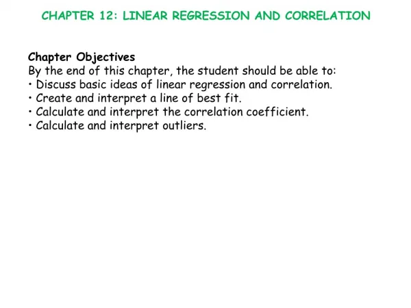
Chapter Goals After completing this chapter, you should be able to: • Calculate and interpret the correlation between two variables • Determine whether the correlation is significant • Calculate and interpret the simple linear regression equation for a set of data • Understand the assumptions behind regression analysis • Determine whether a regression model is significant
Chapter Goals (continued) After completing this chapter, you should be able to: • Calculate and interpret confidence intervals for the regression coefficients • Recognize regression analysis applications for purposes of prediction and description • Recognize some potential problems if regression analysis is used incorrectly
Scatter Plots and Correlation • A scatter plot (or scatter diagram) is used to show the relationship between two quantitative variables • The linear relationship can be: • Positive – as x increases, y increases • As advertising dollars increase, sales increase • Negative – as x increases, y decreases • As expenses increase, net income decreases
Scatter Plot Examples Linear relationships Curvilinear relationships y y x x y y x x
Scatter Plot Examples (continued) Strong relationships Weak relationships y y x x y y x x
Scatter Plot Examples (continued) No relationship y x y x
Correlation Coefficient (continued) • The sample correlation coefficient r is a measure of the strength of the linear relationship between two variables, based on sample observations • Only concerned with strength of the relationship • No causal effect is implied • Causal effect: if event A happens, event B is more likely happen.
Features of r • Range between -1 and 1 • The closer to -1, the stronger the negative linear relationship • The closer to 1, the stronger the positive linear relationship • The closer to 0, the weaker the linear relationship • +1 or -1 are perfect correlations where all data points fall on a straight line
Examples of Approximate r Values y y y x x x r = -1 r = -.6 r = 0 y y x x r = +.3 r = +1
Calculating the Correlation Coefficient Sample correlation coefficient: or the algebraic equivalent: where: r = Sample correlation coefficient n = Sample size x = Value of the independent variable y = Value of the dependent variable
Quick Example • A national consumer magazine reported the following correlations. • The correlation between car weight and car reliability is -0.30. • The correlation between car weight and annual maintenance cost is 0.20. • Heavier cars tend to be less reliable. • Heavier cars tend to cost more to maintain. • Car weight is related more strongly to reliability than to maintenance cost.
Calculation Example (continued) Tree Height, y Scatter Plot r = 0.886 → relatively strong positive linear association between x and y Trunk Diameter, x
Excel Output • Excel Correlation Output • Tools / data analysis / correlation… • Try this using Excel (copy and paste data): refer to the tutorial Correlation between Tree Height and Trunk Diameter
Significance Test for Correlation • Hypotheses H0: ρ = 0 (no correlation) HA: ρ≠ 0 (correlation exists) • t Test statistic (two samples) (with n – 2 degrees of freedom) Assumptions: Data are interval or ratio x and y are normally distributed The Greek letter ρ (rho) represents the population correlation coefficient We lose one more degree of freedom for each sample mean (TWO samples)
Example: Produce Stores Is there evidence of a linear relationship between tree height and trunk diameter at the 0.05 level of significance? H0: ρ (R)= 0 (No correlation) H1: ρ(R)≠ 0 (correlation exists) =0.05 , df=8 - 2 (two sample means) = 6
Produce Stores: Test Solution TINV(6, .05) = 2.4469 P-value: TDIST(4.68, 6, .05) = 0.00396 Decision:Reject H0 Conclusion:There is sufficient evidence of a linear relationship at the 0.05 significance level d.f. = 8-2 = 6 a/2=0.025 a/2=0.025 Reject H0 Do not reject H0 Reject H0 -tα/2 tα/2 0 -2.4469 2.4469 4.68
Regression Analysis(video clip on the website) • Regression analysis is used to: • Predict the value of a dependent variable, such as salesbased on the value of at least one independent variable, such as years at company as a salesmen • Based on the Midwest Excel file • Dependent variable: the variable we wish to explain (cause) • Independent variable: the variable used to explain the dependent variable (effect) • Explain the impact of changes in an independent variable on the dependent variable
Simple Linear Regression Model • Only one independent variable • Relationship between iv and dv is described by a linear function • independent: iv, dependent: dv • Changes in dv are assumed to be caused by changes in iv
Types of Regression Models Positive Linear Relationship Relationship NOT Linear Negative Linear Relationship No Relationship
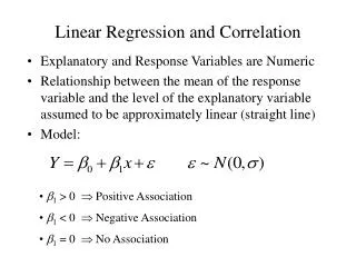
Population Linear Regression The population regression model: Population SlopeCoefficient Population y intercept Independent Variable residual Dependent Variable Linear component Random Error component
Residual • Because a linear regression model is not always appropriate for the data, • the appropriateness of the model can be assessed by defining and examining residuals and residual plots.
Population Linear Regression (continued) y Observed Value of y for xi ei Slope = b1 Predicted Value of y for xi Random Error for this x value Intercept = b0 x xi
Estimated Regression Model The sample regression line provides an estimate of the population regression line Estimated (or predicted) y value Estimate of the regression intercept Estimate of the regression slope Independent variable The individual random error terms ei have a mean of zero
Simple Linear Regression Example • A real estate agent wishes to examine the relationship between the selling price of a home and its size (measured in square feet) • A random sample of 10 houses is selected • “x” variable affects (influences) “y” variable • Dependent variable (y) = house price in $1000s • Independent variable (x) = square feet
Regression Using Excel • Do this together, enter data and select Regression
Excel Output The regression equation is:
Regression Analysis for Prediction: House Prices Estimated Regression Equation: Predict the price for a house with 2000 square feet
Example: House Prices Predict the price for a house with 2000 square feet: The predicted price for a house with 2000 square feet is 317.85($1,000s) = $317,850
Graphical Presentation • House price model: scatter plot and regression line Slope = 0.10977 Intercept = 98.248
Interpretation of the Intercept, b0 • b0 is the estimated average value of Y when the value of X is zero (if x = 0 is in the range of observed x values) • Here, no houses had 0 square feet, so b0 = 98.24833 just indicates that, for houses within the range of sizes observed. $98,248.33 is the portion of the house price not explained by square feet. So, it has no meaning.
Interpretation of the Slope Coefficient, b1 • b1 measures the estimated change in the average value of Y as a result of a one-unit change in X • Here, b1 = 0.10977 tells us that the average value of a house increases by 0.10977($1000) = $109.77, on average, for each additional one square foot of size
Excel Output 58.08% of the variation in house prices is explained by variation in square feet
Explained and Unexplained Variation (page 591-594) • Total variation is made up of two parts: explained unexplained Total sum of Squares Sum of Squares Error Sum of Squares Regression where: = Average value of the dependent variable y = Observed values of the dependent variable = Estimated value of y for the given x value
Coefficient of Determination, R2 • The coefficient of determination is the portion of the total variation in the dependent variable that is explained by variation in the independent variable • The coefficient of determination is also called R-squared and is denoted as R2 where
Coefficient of Determination, R2 (continued) Coefficient of determination Note: In the single independent variable case, the coefficient of determination is where: R2 = Coefficient of determination r = Simple correlation coefficient
Examples of Approximate R2 Values (continued) y R2 = 1 Perfect linear relationship between x and y: 100% of the variation in y is explained by variation in x x y x
Examples of Approximate R2 Values (continued) y 0 < R2 < 1 Weaker linear relationship between x and y: Some but not all of the variation in y is explained by variation in x x y x
Examples of Approximate R2 Values “Linear Regression” on the class website covers up to this slide (#38). R2 = 0 y No linear relationship between x and y: The value of Y does not depend on x. (None of the variation in y is explained by variation in x) x R2 = 0
Significance Tests • For simple linear regression there are there equivalent statistical tests: • Test for significance of the correlation between x and y • Test for significance of the coefficient of determination (r2) • Test for significance of the regression slope coefficient (b1)
Test for Significance of Coefficient of Determination • Hypotheses H0: ρ2 = 0 HA: ρ2≠ 0 • Test statistic • (with D1 = 1 and D2 = n - 2 degrees of freedom) H0: The independent variable does not explain a significant portion of the variation in the dependent variable (in other word, the regression slope is zero) HA: The independent variable does explain a significant portion of the variation in the dependent variable = 0.05
Excel Output The critical F value from Appendix H for = 0.05 and D1 = 1 and D2 = 8 d.f. is 5.318. Since 11.085 > 5.318 we reject H0: ρ2 = 0
Inference about the Slope: t Test (continued) Estimated Regression Equation: The slope of this model is 0.1098 Does square footage of the house affect its sales price?
H0: β1 = 0 HA: β1 0 Inferences about the Slope: tTest Example Test Statistic: t = 3.329 b1 t From Excel output: d.f. = 10-2 = 8 Decision: Conclusion: Reject H0 a/2=0.025 a/2=0.025 There is sufficient evidence that square footage affects house price Reject H0 Do not reject H0 Reject H0 -tα/2 tα/2 0 -2.3060 2.3060 3.329
Regression Analysis for Description Confidence Interval Estimate of the Slope: d.f. = n - 2 Excel Printout for House Prices: At 95% level of confidence, the confidence interval for the slope is (0.0337, 0.1858)
Regression Analysis for Description Since the units of the house price variable is $1000s, we are 95% confident that the average impact on sales price is between $33.70 and $185.80 per square foot of house size This 95% confidence interval does not include 0. Conclusion: There is a significant relationship between house price and square feet at the 0.05 level of significance
Estimation of Mean Values: Example Confidence Interval Estimate for E(y)|xp Find the 95% confidence interval for the average price of 2,000 square-foot houses Predicted Price Yi = 317.85 ($1,000s) The confidence interval endpoints are 280.66 -- 354.90, or from $280,660 -- $354,900
Estimation of Individual Values: Example Prediction Interval Estimate for y|xp Find the 95% confidence interval for an individual house with 2,000 square feet Predicted Price Yi = 317.85 ($1,000s) The prediction interval endpoints are 215.50 -- 420.07, or from $215,500 -- $420,070