Download
1 / 53
580 likes | 1.25k Vues
Chapter 13 Introduction to Linear Regression and Correlation Analysis. Chapter Goals. To understand the methods for displaying and describing relationship among variables. Methods for Studying Relationships. Graphical Scatterplots Line plots 3-D plots Models Linear regression

E N D
Chapter 13Introduction to Linear Regression and Correlation Analysis Fall 2006 – Fundamentals of Business Statistics
Chapter Goals To understand the methods for displaying and describing relationship among variables Fall 2006 – Fundamentals of Business Statistics
Methods for Studying Relationships • Graphical • Scatterplots • Line plots • 3-D plots • Models • Linear regression • Correlations • Frequency tables Fall 2006 – Fundamentals of Business Statistics
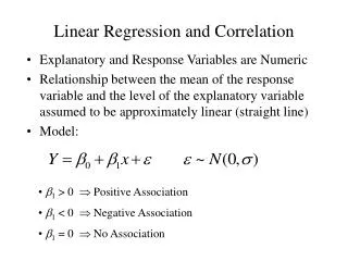
Two Quantitative Variables The response variable, also called the dependent variable, is the variable we want to predict, and is usually denoted by y. The explanatory variable, also called the independent variable, is the variable that attempts to explain the response, and is denoted by x. Fall 2006 – Fundamentals of Business Statistics
YDI 7.1 Fall 2006 – Fundamentals of Business Statistics
Scatter Plots and Correlation • A scatter plot (or scatter diagram) is used to show the relationship between two variables • Correlation analysis is used to measure strength of the association (linear relationship) between two variables • Only concerned with strength of the relationship • No causal effect is implied Fall 2006 – Fundamentals of Business Statistics
Example • The following graph shows the scatterplot of Exam 1 score (x) and Exam 2 score (y) for 354 students in a class. Is there a relationship? Fall 2006 – Fundamentals of Business Statistics
Scatter Plot Examples Linear relationships Curvilinear relationships y y x x y y x x Fall 2006 – Fundamentals of Business Statistics
Scatter Plot Examples (continued) No relationship y x y x Fall 2006 – Fundamentals of Business Statistics
Correlation Coefficient • The population correlation coefficient ρ (rho) measures the strength of the association between the variables • The sample correlation coefficient r is an estimate of ρ and is used to measure the strength of the linear relationship in the sample observations (continued) Fall 2006 – Fundamentals of Business Statistics
Features of ρand r • Unit free • Range between -1 and 1 • The closer to -1, the stronger the negative linear relationship • The closer to 1, the stronger the positive linear relationship • The closer to 0, the weaker the linear relationship Fall 2006 – Fundamentals of Business Statistics
Examples of Approximate r Values Tag with appropriate value: -1, -.6, 0, +.3, 1 y y y x x x y y x x Fall 2006 – Fundamentals of Business Statistics
Earlier Example Fall 2006 – Fundamentals of Business Statistics
YDI 7.3 What kind of relationship would you expect in the following situations: • age (in years) of a car, and its price. • number of calories consumed per day and weight. • height and IQ of a person. Fall 2006 – Fundamentals of Business Statistics
YDI 7.4 Identify the two variables that vary and decide which should be the independent variable and which should be the dependent variable. Sketch a graph that you think best represents the relationship between the two variables. • The size of a persons vocabulary over his or her lifetime. • The distance from the ceiling to the tip of the minute hand of a clock hung on the wall. Fall 2006 – Fundamentals of Business Statistics
Introduction to Regression Analysis • Regression analysis is used to: • Predict the value of a dependent variable based on the value of at least one independent variable • Explain the impact of changes in an independent variable on the dependent variable Dependent variable: the variable we wish to explain Independent variable: the variable used to explain the dependent variable Fall 2006 – Fundamentals of Business Statistics
Simple Linear Regression Model • Only one independent variable, x • Relationship between x and y is described by a linear function • Changes in y are assumed to be caused by changes in x Fall 2006 – Fundamentals of Business Statistics
Types of Regression Models Positive Linear Relationship Relationship NOT Linear Negative Linear Relationship No Relationship Fall 2006 – Fundamentals of Business Statistics
Population Linear Regression The population regression model: Random Error term, or residual Population SlopeCoefficient Population y intercept Independent Variable Dependent Variable Linear component Random Error component Fall 2006 – Fundamentals of Business Statistics
Linear Regression Assumptions • Error values (ε) are statistically independent • Error values are normally distributed for any given value of x • The probability distribution of the errors is normal • The probability distribution of the errors has constant variance • The underlying relationship between the x variable and the y variable is linear Fall 2006 – Fundamentals of Business Statistics
Population Linear Regression (continued) y Observed Value of y for xi εi Slope = β1 Predicted Value of y for xi Random Error for this x value Intercept = β0 x xi Fall 2006 – Fundamentals of Business Statistics
Estimated Regression Model The sample regression line provides an estimate of the population regression line Estimated (or predicted) y value Estimate of the regression intercept Estimate of the regression slope Independent variable The individual random error terms ei have a mean of zero Fall 2006 – Fundamentals of Business Statistics
Earlier Example Fall 2006 – Fundamentals of Business Statistics
Residual A residual is the difference between the observed response y and the predicted response ŷ. Thus, for each pair of observations (xi, yi), the ith residual isei= yi− ŷi= yi− (b0+ b1x) Fall 2006 – Fundamentals of Business Statistics
Least Squares Criterion • b0 and b1 are obtained by finding the values of b0 and b1 that minimize the sum of the squared residuals Fall 2006 – Fundamentals of Business Statistics
Interpretation of the Slope and the Intercept • b0 is the estimated average value of y when the value of x is zero • b1 is the estimated change in the average value of y as a result of a one-unit change in x Fall 2006 – Fundamentals of Business Statistics
The Least Squares Equation • The formulas for b1 and b0 are: algebraic equivalent: and Fall 2006 – Fundamentals of Business Statistics
Finding the Least Squares Equation • The coefficients b0 and b1 will usually be found using computer software, such as Excel, Minitab, or SPSS. • Other regression measures will also be computed as part of computer-based regression analysis Fall 2006 – Fundamentals of Business Statistics
Simple Linear Regression Example • A real estate agent wishes to examine the relationship between the selling price of a home and its size (measured in square feet) • A random sample of 10 houses is selected • Dependent variable (y) = house price in $1000s • Independent variable (x) = square feet Fall 2006 – Fundamentals of Business Statistics
Sample Data for House Price Model Fall 2006 – Fundamentals of Business Statistics
SPSS Output The regression equation is: Fall 2006 – Fundamentals of Business Statistics
Graphical Presentation • House price model: scatter plot and regression line Slope = 0.110 Intercept = 98.248 Fall 2006 – Fundamentals of Business Statistics
Interpretation of the Intercept, b0 • b0 is the estimated average value of Y when the value of X is zero (if x = 0 is in the range of observed x values) • Here, no houses had 0 square feet, so b0 = 98.24833 just indicates that, for houses within the range of sizes observed, $98,248.33 is the portion of the house price not explained by square feet Fall 2006 – Fundamentals of Business Statistics
Interpretation of the Slope Coefficient, b1 • b1 measures the estimated change in the average value of Y as a result of a one-unit change in X • Here, b1 = .10977 tells us that the average value of a house increases by .10977($1000) = $109.77, on average, for each additional one square foot of size Fall 2006 – Fundamentals of Business Statistics
Least Squares Regression Properties • The sum of the residuals from the least squares regression line is 0 ( ) • The sum of the squared residuals is a minimum (minimized ) • The simple regression line always passes through the mean of the y variable and the mean of the x variable • The least squares coefficients are unbiased estimates of β0 and β1 Fall 2006 – Fundamentals of Business Statistics
YDI 7.6 The growth of children from early childhood through adolescence generally follows a linear pattern. Data on the heights of female Americans during childhood, from four to nine years old, were compiled and the least squares regression line was obtained as ŷ= 32 + 2.4x where ŷis the predicted height in inches, and x is age in years. • Interpret the value of the estimated slope b1= 2. 4. • Would interpretation of the value of the estimated y-intercept, b0= 32, make sense here? • What would you predict the height to be for a female American at 8 years old? • What would you predict the height to be for a female American at 25 years old? How does the quality of this answer compare to the previous question? Fall 2006 – Fundamentals of Business Statistics
Coefficient of Determination, R2 • The coefficient of determination is the portion of the total variation in the dependent variable that is explained by variation in the independent variable • The coefficient of determination is also called R-squared and is denoted as R2 Fall 2006 – Fundamentals of Business Statistics
Coefficient of Determination, R2 (continued) Note: In the single independent variable case, the coefficient of determination is where: R2 = Coefficient of determination r = Simple correlation coefficient Fall 2006 – Fundamentals of Business Statistics
Examples of Approximate R2 Values y y x x y y x x Fall 2006 – Fundamentals of Business Statistics
Examples of Approximate R2 Values R2 = 0 y No linear relationship between x and y: The value of Y does not depend on x. (None of the variation in y is explained by variation in x) x R2 = 0 Fall 2006 – Fundamentals of Business Statistics
SPSS Output Fall 2006 – Fundamentals of Business Statistics
Standard Error of Estimate • The standard deviation of the variation of observations around the regression line is called the standard error of estimate • The standard error of the regression slope coefficient (b1) is given by sb1 Fall 2006 – Fundamentals of Business Statistics
SPSS Output Fall 2006 – Fundamentals of Business Statistics
Comparing Standard Errors Variation of observed y values from the regression line Variation in the slope of regression lines from different possible samples y y x x y y x x Fall 2006 – Fundamentals of Business Statistics
Inference about the Slope: t Test • t test for a population slope • Is there a linear relationship between x and y? • Null and alternative hypotheses • H0: β1 = 0 (no linear relationship) • H1: β1 0 (linear relationship does exist) • Test statistic where: b1 = Sample regression slope coefficient β1 = Hypothesized slope sb1 = Estimator of the standard error of the slope Fall 2006 – Fundamentals of Business Statistics
Inference about the Slope: t Test (continued) Estimated Regression Equation: The slope of this model is 0.1098 Does square footage of the house affect its sales price? Fall 2006 – Fundamentals of Business Statistics
H0: β1 = 0 HA: β1 0 Inferences about the Slope: tTest Example Test Statistic: t = 3.329 b1 t From Excel output: d.f. = 10-2 = 8 Decision: Conclusion: Reject H0 a/2=.025 a/2=.025 There is sufficient evidence that square footage affects house price Reject H0 Do not reject H0 Reject H0 -tα/2 t(1-α/2) 0 -2.3060 2.3060 3.329 Fall 2006 – Fundamentals of Business Statistics
Regression Analysis for Description Confidence Interval Estimate of the Slope: d.f. = n - 2 Excel Printout for House Prices: At 95% level of confidence, the confidence interval for the slope is (0.0337, 0.1858) Fall 2006 – Fundamentals of Business Statistics
Regression Analysis for Description Since the units of the house price variable is $1000s, we are 95% confident that the average impact on sales price is between $33.70 and $185.80 per square foot of house size This 95% confidence interval does not include 0. Conclusion: There is a significant relationship between house price and square feet at the .05 level of significance Fall 2006 – Fundamentals of Business Statistics
Residual Analysis • Purposes • Examine for linearity assumption • Examine for constant variance for all levels of x • Evaluate normal distribution assumption • Graphical Analysis of Residuals • Can plot residuals vs. x • Can create histogram of residuals to check for normality Fall 2006 – Fundamentals of Business Statistics