FAULTING & DEFORMATION
FAULTING & DEFORMATION. Dinosaur National Monument, Utah, USA. Material is perfectly elastic until it undergoes brittle fracture when applied stress reaches f Material undergoes plastic deformation when stress exceeds yield stress 0

FAULTING & DEFORMATION
E N D
Presentation Transcript
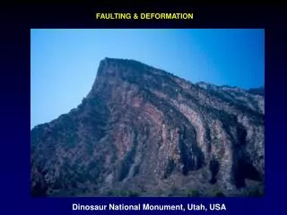
FAULTING & DEFORMATION Dinosaur National Monument, Utah, USA
Material is perfectly elastic until it undergoes brittle fracture when applied stress reaches f Material undergoes plastic deformation when stress exceeds yield stress 0 Permanent strain results from plastic deformation when stress is raised to 0 ‘and released
AT LOW PRESSURES ROCKS ARE BRITTLE, BUT AT HIGH PRESSURES THEY BEHAVE DUCTILY, OR FLOW Consider rock subjected to compressive stress that exceeds a confining pressure For confining pressures less than about 4 Kb material behaves brittlely - it reaches the yield strength and then fails For higher confining pressures material flows ductilely. These pressures occur not far below the earth's surface - 3 km depth corresponds to a kilobar pressure - so 8 Kb is reached at about 24 km This experimental result is consistent with the idea of strong lithosphereunderlain by the weaker asthenosphere Note: 1 MPa = 10 b ; 100 MPa = 1 Kb Kirby, 1980
Note: compressive stress convention Positive in rock mechanics Negative in seismology (outward normal vector) SHEAR NORMAL
Laboratory experiments on rocks under compression show that fracture occurs when a critical combination of the absolute value of shear stress and the normal stress is exceeded. Higher normal stress requires higher shear stress for fracture This relation, the Coulomb-Mohr failure criterion, is | | = o -n where oand n are material properties known as the cohesive strength and coefficient of internal friction. INCREASED STRESS BREAKS ROCK WHEN MOHR’S CIRCLE REACHES COULOMB-MOHR FAILURE CRITERION Often: for given normal stress, rock breaks when shear stress high enough
MOHR’S CIRCLE AND COULOMB-MOHR FAILURE CRITERION DETERMINE Failure plane given by angle Failure stress given by point F
CONVERSELY, CAN FIND STRESS IN EARTH WHEN FAILURE OCCURS FROM ANGLE OF FAILURE PLANE
With no internal friction, fracture occurs at an angle of 45º. With no internal friction, e.g. n=1, fracture angle is 67.5º, and fault plane is closer (22.5 º) to the maximum compression (1 ) direction.
MOHR'S CIRCLE FOR SLIDING ON ROCK'S PREEXISTING FAULTS Preexisting faults have no cohesive strength Lower shear stress required for slip New fracture would form at an angle f given by fracture line. However, slip will occur on any preexisting fault with angle between S1 and S2 given by intersection of the circle with frictional sliding line. If so, as stress increases, sliding favored over new fault formation
SEISMOLOGICAL CONSEQUENCE: P AXES FROM FOCAL MECHANISMS ON PREEXISTING FAULT DO NOT ONLY REFLECT STRESS DIRECTION Ni and Barazangi, 1984 Thrust focal mechanisms along Himalayan front have fault planes that rotate as trend of the mountains changes, suggesting that fault planes are controlled by the existing structures so P axes only partially reflect stress field. When stress axes inferred from many fault plane solutions in an area seem relatively coherent, assume the crust contains preexisting faults of all orientations, so average stress orientation inferred from focal mechanisms is not seriously biased.
PORE PRESSURE EFFECTS _ Water and other fluids are often present in rocks, especially in the upper crust.The fluid pressure, known as pore pressure, reduces the effect of the normal stress and allows sliding to take place at lower shear stresses. This is modeled by replacing normal stress with the effective normal stress = - P f , where Pf is the pore fluid pressure. Similarly, taking into account pore pressure, effective principal stresses 1 = 1 - Pf2 = 2 - Pf are used in the fracture theory. The role of pore pressure in making sliding easier can be seen by trying to slide an object across a dry table and then wetting the table _ _
Laboratory results for sliding on existing faults of various rock types find relation between normal stress on fault and shear stress required for sliding Byerlee's Law: Byerlee, 1978
Byerlee’s law, relating normal and shear stresses on a fault, can be used to infer principal stress as a function of depth. Assume the crust contains faults of all orientations, and the stresses cannot exceed the point where Mohr's circle is tangent to the frictional sliding line, or else sliding will occur
USING BYERLEE’S LAW AND MOHR’S CIRCLE RELATES PRINCIPAL STRESSES AS A FUNCTION OF PRESSURE AND HENCE DEPTH
STRENGTH OF THE CRUST H - v MAXIMUM DIFFERENCE BETWEEN HORIZONTAL AND VERTICAL STRESSES THAT ROCK CAN SUPPORT STRENGTH IN EXTENSION
STRENGTH OF THE CRUST H - v MAXIMUM DIFFERENCE BETWEEN HORIZONTAL AND VERTICAL STRESSES THAT ROCK CAN SUPPORT STRENGTH IN COMPRESSION
HORIZONTAL STRESSES MEASURED IN SOUTHERN AFRICA Dots are for horizontal stresses being the least compressive (3), and triangles are for horizontal stresses being the most compressive (1). The lithostatic stress gradient (26.5 MPa/km) is shown, along with Byerlee's law (BY) for hydrostatic pore pressure (HYD) and zero pore pressure (DRY). Stronger lines are for compression, and weaker ones are for extension. Observed stresses are within the maximum and minimum BY-DRY lines. Brace and Kohlstedt, 1980
When rocks behave brittlely their behavior is not time-dependent; they either strain elastically or fail In contrast, ductile rock deforms over time A common model for the time-dependent behavior is a Maxwell viscoelastic material, which behaves like an elastic solid on short time scales and like a viscous fluid on long time scales. This model can describe the mantle, because seismic waves propagate as though the mantle were solid, whereas postglacial rebound and mantle convection occur as though the mantle were fluid. Stress proportional to strain Stress proportional to strain rate
MAXWELL VISCOELASTIC SUBSTANCE Consider elastic material as a spring, which exerts a force proportional to distance. Thus stress and strain are proportional at any instant, and there are no time-dependent effects. In contrast, a viscous material is thought of as a dashpot, a fluid damper that exerts a force proportional to velocity. Hence stress and strain rate are proportional, and the material's response varies with time. These effects are combined in a viscoelastic material, which can be thought of as a spring and dashpot in series
MAXWELL VISCOELASTIC SUBSTANCE STRESS RESPONSE TO STRAIN APPLIED AT T=0 THAT REMAINS CONSTANT Stress relaxes from initial value
MAXWELL VISCOELASTIC SUBSTANCE Stress decay
If we model the mantle as viscoelastic, then a load applied on the surface has an effect that varies with time. Initially, the earth responds elastically, causing large flexural bending stresses. With time, the mantle flows, so the deflection beneath the load deepens and stresses relax. In the time limit, stress goes to zero and the deflection approaches the isostatic solution because isostasy amounts to assuming the lithosphere has no strength. Stress relaxation may explain why large earthquakes are rare at continental margins, except where glacial loads have been recently removed Although the large sediment loads should produce stresses much greater than other sources of intraplate stress including the less dense ice loads, the stresses produced by sediment loading early in the margin's history may have relaxed. Stein et al., 1989 Response to a 150-km wide sediment load at a passive margin
Viscosity decrease with temperature is assumed to give rise to strong lithosphere overlying weaker asthenosphere, and the restriction of earthquakes to shallow depths
STRENGTH OF THE LITHOSPHERE The strength of the lithosphere as a function of depth depends upon the deformation mechanism. At shallow depths rocks fail either by brittle fracture or frictional sliding on preexisting faults. Both processes depend in a similar way on the normal stress, with rock strength increasing with depth. At greater depths the ductile flow strength of rocks is less than the brittle or frictional strength, so the strength is given by the flow laws and decreases with depth as the temperatures increase. This temperature-dependent strength is the reason that the cold lithosphere forms the planet's strong outer layer. To calculate the strength, a strain rate and a geothermal gradient giving temperature as a function of depth are assumed
Strength envelope gives strength vs depth Shows effects of material, pore pressure, geotherm, strain rate BRITTLE DUCTILE Brace & Kohlstedt, 1980 Strength increases with depth in the brittle region due to the increasing normal stress, and then decreases with depth in the ductile region due to increasing temperature. Hence strength is highest at the brittle-ductile transition. Strength decreases rapidly below this transition, so the lithosphere should have little strength at depths > ~25 km in the continents and 50 km in the oceans.
Strength & depth of brittle-ductile transition vary Olivine is stronger in ductile flow than quartz, so oceanic lithosphere is stronger than continental BRITTLE DUCTILE Brace & Kohlstedt, 1980 Higher pore pressures reduce strength Lithosphere is stronger for compression than for tension in the brittle regime, but symmetric in the ductile regime.
Cooling of oceanic lithosphere with age also increases rock strength and seismic velocity. Thus elastic thickness of the lithosphere inferred from the deflection caused by loads such as seamounts , maximum depth of intraplate earthquakes within the oceanic lithosphere , & depth to the low velocity zone determined from surface wave dispersion all increase with age. Stein and Stein, 1992
STRENGTH VERSUS AGE IN COOLING OCEANIC LITHOSPHERE As oceanic lithosphere ages and cools, the predicted strong region deepens. This seems plausible since earthquake depths, seismic velocities, and effective elastic thicknesses imply the strong upper part of the lithosphere thickens with age Wiens and Stein, 1983
STRENGTH VERSUS AGE IN COOLING OCEANIC LITHOSPHERE Strength envelopes are consistent with the observation that the maximum depth of earthquakes in oceanic lithosphere is approximately bounded by the 750\(deC isotherm. This makes sense, because for a given strain rate and rheology the exponential dependence on temperature would make a limiting strength for seismicity approximate a limiting temperature. Wiens and Stein, 1985
Earthquake limiting temperatures for continental seismicity are much lower than those for oceanic lithosphere, since the quartz rheology in continents is much weaker than olivine. Strehlau & Meissner
"JELLY SANDWICH" STRENGTH PROFILE FOR CONTINENTS In continental lithosphere strength in the quartz-rich crust increases with depth and then decreases. Below the Moho there should be a second, deeper, zone of strength due to the olivine rheology. This profile including a weak zone may be part of the reason why continents deform differently than oceanic lithosphere. For example, some continental mountain building may involve crustal thickening in which slices of upper crust, which are too buoyant to subduct, are instead thrust atop one another. The weaker lower crust may contribute in other ways to the general phenomenon that continental plate boundaries are broader and more complex than oceanic ones Chen and Molnar, 1983
EARTHQUAKES & ROCK FRICTION It is natural to assume that earthquakes occur when tectonic stress exceeds the strength, so a new fault forms or an existing one slips. Thus steady motion across a plate boundary seems likely to give a cycle of successive earthquakes at regular intervals, with the same slip and stress drop However, we have seen that the earthquake history is more complicated. Shimazaki and Nakata, 1980
The time between earthquakes on plate boundaries varies although the plate motion causing the earthquakes is steady Earthquakes sometimes rupture the same segments of a boundary as in earlier earthquakes, and other times along a different set Many large earthquakes show a complex rupture, parts of the fault releasing more seismic energy than others Attempts to understand these complexities often combine two basic themes. Some of the complexity may be due to intrinsic randomness of the failure process, such that some small ruptures cascade into large earthquakes, whereas others do not. Other aspects of complexity may be due to features of rock friction. GAP? NOTHING YET Ando, 1975
EXPERIMENT: STRESS APPLIED UNTIL ROCK BREAKS: STICK SLIP OCCURS When the fault forms, some of the stress is released and motion stops. If stress is reapplied, another stress drop and motion occur once stress reaches a certain level. As stress is reapplied, jerky sliding and stress release continues This pattern, called stick-slip, looks like a laboratory version of a sequence of earthquakes on a fault. By this analogy, the stress drop in an earthquake relieves only part of the total tectonic stress, and as the fault continues to be loaded by tectonic stress, occasional earthquakes occur. The analogy is strengthened by the fact that at higher temperatures (about 300° for granite), stick-slip does not occur Instead, stable sliding occurs on the fault, much as earthquakes do not occur at depths where the temperature exceeds a certain value. STICK SLIP STABLE SLIDING Brace and Byerlee, 1970
Stick-slip results from a familiar phenomenon - it’s harder to start an object sliding against friction than to keep it going once it’s sliding. This is because the static friction stopping the object from sliding exceeds the dynamic friction that opposes motion once sliding starts Thus a steady load, combined with the difference in static and dynamic friction, causes an instability and a sequence of discrete slip events. To understand how this difference causes stick-slip, and get insight into stick-slip as a model for earthquakes, note that if an object is pulled across a table with a rubber band, jerky stick-slip motion occurs This effect is the basis of cross-country skiing: loading one ski makes it grip the snow while unloading the other lets it glide.
Slider loaded by force f due to spring end moving at velocity v Before sliding, block is retarded by static friction force = - s, the product of normal stress due to the block's weight, and the static friction coefficient s Once sliding starts friction force decreases to d where dis the smaller dynamic friction As spring shortens force decreases until it becomes less than retarding friction Series of slip events occur, each with slip ∆u and force change ∆f (stress drop) SLIDER BLOCK AND SPRING MODEL FOR STICK-SLIP AS AN EARTHQUAKE MECHANISM
Earthquake cycle for a model in which a strike-slip fault with rate- and state- dependent frictional properties is loaded by plate motion Tse and Rice, 1986 The slip history for three cycles as a function of depth and time is shown by the lines, each of which represents a specific time. Steady motion occurs at depth, and stick-slip occurs above 11 km. Such models replicate many aspects of the earthquake cycle. An Interesting difference, however, is that the models predict earthquakes at regular intervals, whereas earthquake histories are quite variable.
SOME VARIABILITY MAY BE DUE TO THE EFFECTS OF EARTHQUAKES ON OTHER FAULTS, OR OTHER SEGMENTS OF THE SAME FAULT To include this in the slider model, assume that after an earthquake cycle, the compressive normal stress on the slider is reduced. This "unclamping" reduces the frictional force resisting sliding, so it takes less time for the spring force to rise again to the level needed for the next slip event. Conversely, increased compression "clamps" the slider more, and increases the time to the next slip event. In addition, the stress drop in the slip event changes when changes Stress changes can make earthquake sooner or more likely
EARTHQUAKE OBSERVATIONS PROVIDE SUPPORT FOR STRESS TRIGGERING Failure is favored when Coulomb failure stress = + increases Changes in Los Angeles region due to the 1971 (Ms 6.6) San Fernando earthquake reflect the focal mechanism, thrust faulting on NW-SE striking fault. Two moderate earthquakes, 1987 Whittier Narrows (ML 5.9) and 1994 Northridge (Ms 6.7), subsequently occurred where the 1971 earthquake increased the failure stress, suggesting the stress change may have had a role in triggering the earthquakes. Stein et al., 1994 A similar pattern has been found after other earthquakes, and some studies have found aftershocks concentrated in regions where the main shock increased the failure stress.
Stress triggering may explain why successive earthquakes on a fault sometimes seem to have a coherent pattern. The 1999 Ms 7.4 Izmit earthquake on the North Anatolian fault appears to be part of a sequence of major (Ms 7) earthquakes over the past 60 years, which occurred successively further to the west and closer to the city of Istanbul The Izmit earthquake and the November 1999 Ms 7.1 Duzce earthquakes increased failure stress near Istanbul Parsons et al., 2000
1906 San Francisco earthquake may have reduced failure stress on other faults in the area, causing a "stress shadow" and increasing the expected time until the next earthquake on these faults. This is consistent with the observation that in 75 years before the 1906 earthquake, the area had 14 earthquakes with Mw > 6, whereas only one occurred since Stress change SAF USGS
WHAT IS THE STRESS ON FAULTS? Major issue for seismology & tectonics In Coulomb stress models, predicted stress changes are ~ 1 bar, or only 1-10% of typical earthquake stress drops. Such small changes should only trigger an earthquake if tectonic stress is already close to failure. Earthquake stress drops estimated from seismology are typically less than a few hundred bars (a few MPa). However, expected strength of the lithosphere from lab results is much higher, in the kilobar (hundreds of MPa) range. The laboratory results and frictional models suggest an explanation for this difference, because in both the stress drop during a slip event is only a fraction of the total stress Even so, major problem remains
"SAN ANDREAS" OR "FAULT STRENGTH" PARADOX Fault under shear stress slipping at rate v should generate fractional heat at a rate equal to v . Thus if shear stresses on faults are as high (Kb or hundreds of MPa) as expected from strength envelopes, significant heat should be produced. However, little if any heat flow anomaly is found across the San Andreas suggesting the fault is much weaker than expected. Lachenbruch and Sass, 1988
Although Coulomb-Mohr model predicts that maximum principal stress directions inferred from focal mechanisms, geological data, and boreholes ~ 23° from the San Andreas fault, observed directions are essentially perpendicular to the fault, implying that the fault acts almost like a free surface. There is no generally accepted explanation for these observations. One is that effective stress fault is reduced by high pore pressure, but don’t know if pressures much higher than hydrostatic could be maintained in the fault zone. An alternative is that the fault zone is filled by weak clay-rich gouge, but experiments find that this has normal strength unless pore pressures are high. STRESS ORIENTATIONS ALSO IMPLY WEAK FAULT Zoback et. al, 1989
TREAT LITHOSPHERE AS VISCOUS FLUID Interpolate smoothed geodetic & geologic velocity field Determine effective viscosity by dividing the magnitude of the deviatoric stress tensor by the magnitude of the strain rate tensor Shows deforming vs rigid regions Flesch et al., 2000
VISCOUS FLUID MODEL FOR TIMESCALE DEPENDANT DEFORMATION Frictional plates model effects of earthquake cycle at the trench Dashpot and spring make Maxwell viscoelastic body with both viscous flow leading to permanent deformation and elastic strain that will be recovered by earthquakes (sliding offrictional plates) GPS records instantaneous velocity Geology records long-term rate Liu et al., 2000 GPS Earthquake
VISCOUS FLUID MODELS FOR PARTS OF THE EARTHQUAKE CYCLE Shear strain rate near portions of the San Andreas fault compared to time since last great earthquake. Data similar to the predictions of two alternative models: viscoelastic stress relaxation (solid curve) and aseismic post-seismic slip beneath earthquake fault plane (dashed line). Thatcher,1983
Integration of plate motion, seismological, geodetic & other geophysical and geological data, with lab results & modeling, gives insight into lithospheric process Lots remains to be done Many basic issues unresolved