6. Elastic-Plastic Fracture Mechanics

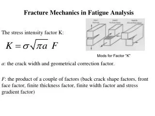
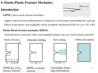
1. 6. Elastic-Plastic Fracture Mechanics Plastic zone crack B L a D Introduction LEFM: Linear elastic fracture mechanics Applies when non-linear deformation is confined to a small region surrounding the crack tip Effects of the plastic zone negligible, linear asymptotic mechanical field (see eqs 4.36, 4.40). Elastic-Plastic fracture mechanics (EPFM) : Generalization to materials with a non-negligible plastic zone size: elastic-plastic materials Diffuse dissipation Elastic Fracture Full yielding Contained yielding LEFM, KIC or GIC fracture criterion Catastrophic failure, large deformations EPFM, JC fracture criterion

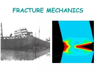
2. Plastic zones (dark regions) in a steel cracked plate (B  5.9 mm): Halfway between surface/midsection Surface of the specimen Midsection • Plastic zones (light regions) in a steel cracked plate (B  5.0 mm): Slip bands at 45° Plane stress dominant Net section stress  0.9 yield stress in both cases.

3. Outline 6.1 Models for small scale yielding : - Estimation of the plastic zonesize using the von Mises yield criterion. - Irwin’s approach (plastic correction). - Dugdale’s model or the strip yield model. 6.2 CTOD as yield criterion. 6.3 The J contour integral as yield criterion. 6.4 Elastoplastic asymptotic field (HRR theory). 6.5 Applications for some geometries (mode I loading).

4. y r θ O x 6.1 Models for small scale yielding : Estimation of the plastic zone size • Von Mises equation: se is the effective stress and si (i=1,2,3) are the principal normal stresses. • Recall the mode I asymptotic stresses in Cartesian components, i.e. LEFM analysis prediction: KI : mode I stress intensity factor (SIF)

5. y r θ O x and in their polar form: Expressions are given in (4.36). We have the relationships (1), and Thus, for the (mode I) asymptotic stress field:

6. Substituting into the expression of se for plane stress Similarly, for plane strain (see expression of sY2p 6.7 )

7. Yielding occurs when: is the uniaxial yield strength increasing n= 0.1, 0.2, 0.3, 0.4, 0.5 • Using theprevious expressions (2) of se and solving for r, plane stress plane strain • Plot of the crack-tip plastic zone shapes (mode I): Plane strain Plane stress (n= 0.0)

8. Remarks: 1) 1D approximation (3)L corresponding to Thus, in plane strain: in plane stress: Triaxial state of stress near the crack tip: Evolution of the plastic zone shape through the thickness: B 2) Significant difference in the size and shape of mode I plastic zones. For a cracked specimen with finite thickness B, effects of the boundaries: - Essentially plane strain in the in the central region. - Pure plane stress state only at the free surface.

9. Stress equilibrium not respected. Alternatively, Irwin plasticity correction using an effective crack length … 3) Similar approach to obtain mode II and III plastic zones: 4) Solutions for rp not strictly correct, because they are based on a purely elastic:

10. The Irwin approach s yy r2 ? r1: Intersection between the elastic distribution and the horizontal line • Mode I loading of a elastic-perfectly plastic material: Elastic: (1) Plane stress assumed (1) (2) Plastic correction (2) crack x r1 r2 To equilibrate the two stresses distributions (cross-hatched region)

11. fictitious crack X • In plane strain, increasing of sY. : Irwin suggested in place of sY • Redistribution of stress due to plastic deformation: Plastic zone length (plane stress): real crack x • Irwin’s model = simplified model for the extent of the plastic zone: - Focus only on the extent of the plastic zone along the crack axis, not on its shape. - Equilibrium condition along the y-axis not respected. • Stress Intensity Factor corresponding to theeffective crack of length aeff=a+r1 (effective SIF)

12. Application: Through-crack in an infinite plate (Irwin, plane stress) with ry ry aeff Solving, closed-form solution: Effective crack length 2 (a+ry) 2a

13. More generally, an iterative process is used to obtain the effective SIF: Initial: Do i = 1, imax : No Yes Y: dimensionless function depending on the geometry. Algorithm: Convergence after a few iterations… Application: Through-crack in an infinite plate (plane stress): s∞= 2 MPa, sY = 50 MPa, a = 0.1 m KI = 1.1209982 4 iterations Keff= 1.1214469

14. Dugdale / Barenblatt yield strip model Very thin plates, with elastic- perfect plastic behavior c c 2a application of the principle of superposition (see chap 5) • Assumptions: Long, slender plastic zone from both crack tips. Perfect plasticity (non-hardening material), plane stress Crack length: 2(a+c) Plastic zone extent • Elastic-plastic behavior modeled by superimposing two elastic solutions: Remote tension + closure stresses at the crack

15. c c • No stress singularity (i.e. terms in ) at the crack tip • Principle: 2a Stresses should be finite in the yield zone: • Length c such that the SIF from the remote tension and closure stress cancel one another • SIF from the remote tension:

16. A B Closure force at a point x in strip-yield zone: x a c Recall first, crack tip A • SIF from the closure stress (see eqs 5.3) crack tip B Total SIF at A: (see equation 5.5) By changing the variable x = -u, the first integral becomes,

17. Thus, KIA can written (see eq. 6.15) The same expression is obtained for KIB (at point B): We denote KIfor KIAor KIB thereafter.

18. Recall that, The SIF of the remote stress must balance with the one due to the closure stress, i.e. By Taylor series expansion of cosines, Irwin and Dugdale approaches predict similar plastic zone sizes. Thus, Keeping only the first two terms, solving for c 1/p = 0.318 and p/8 = 0.392

19. -By setting • Estimation of the effective stress intensity factor with the strip yield model: Thus, and tends to overestimate Keff because the actual aeff less than a+c - Burdekin and Stone derived a more realistic estimation: (see Anderson, third ed., p65)