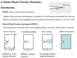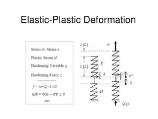
Elastic-Plastic Fracture Mechanics
420 likes | 1.67k Vues
Elastic-Plastic Fracture Mechanics. Introduction When does one need to use LEFM and EPFM? What is the concept of small-scale and large-scale yielding?. Background Knowledge Theory of Plasticity (Yield criteria, Hardening rules) Concept of K, G and K-dominated regions

Elastic-Plastic Fracture Mechanics
E N D
Presentation Transcript
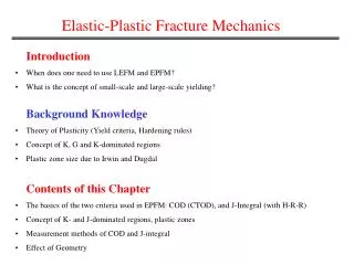
Elastic-Plastic Fracture Mechanics • Introduction • When does one need to use LEFM and EPFM? • What is the concept of small-scale and large-scale yielding? • Background Knowledge • Theory of Plasticity (Yield criteria, Hardening rules) • Concept of K, G and K-dominated regions • Plastic zone size due to Irwin and Dugdal • Contents of this Chapter • The basics of the two criteria used in EPFM: COD (CTOD), and J-Integral (with H-R-R) • Concept of K- and J-dominated regions, plastic zones • Measurement methods of COD and J-integral • Effect of Geometry
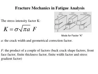
LEFM and EPFM • LEFM • In LEFM, the crack tip stress and displacement field can be uniquely characterized by K, the stress intensity factor. It is neither the magnitude of stress or strain, but a unique parameter that describes the effect of loading at the crack tip region and the resistance of the material. K filed is valid for a small region around the crack tip. It depends on both the values of stress and crack size. We noted that when a far field stress acts on an edge crack of width “a” then for mode I, plane strain case
LEFM cont. For =0 Singularity dominated region LEFM concepts are valid if the plastic zone ismuch smaller than the singularity zones. Irwin estimates Dugdale strip yield model: ASTM: a,B, W-a 2.5 , i.e. of specimen dimension.
EPFM • In EPFM, the crack tip undergoes significant plasticity as seen in the following diagram.
EPFM cont. • EPFM applies to elastoc-rate-independent materials, generally in the large-scale plastic deformation. • Two parameters are generally used: • Crack opening displacement(COD) or crack tip opening displacement (CTOD). • J-integral. • Both these parameters give geometry independent measure of fracture toughness. y x Sharp crack Blunting crack ds
EPFM cont. • Wells discovered that Kic measurements in structural steels required very large thicknesses for LEFM condition. • --- Crack face moved away prior to fracture. • --- Plastic deformation blunted the sharp crack. Note: since Sharp crack Blunting crack • Irwin showed that crack tip plasticity makes the crack behave as if it were longer, say from size a to a + rp • -----plane stress • From Table 2.2, • Set ,
CTOD and strain-energy release rate • Equation relates CTOD () to G for small-scale yielding. Wells proved that • Can valid even for large scale yielding, and is later shown to be related to J. • can also be analyzed using Dugdales strip yield model. If “ ” is the opening at the end of the strip. Consider an infinite plate with a image crack subject to a Expanding in an infinite series, If , and can be given as: In general,
Alternative definition of CTOD Blunting crack Sharp crack Blunting crack Displacement at the original crack tip Displacement at 900 line intersection, suggested by Rice CTOD measurement using three-point bend specimen displacement Vp expanding ' ' '
Elastic-plastic analysis of three-point bend specimen V,P Where is rotational factor, which equates 0.44 for SENT specimen. • Specified by ASTM E1290-89 • --- can be done by both compact tension, and SENT specimen • Cross section can be rectangular or W=2B; square W=B • KI is given by
CTOD analysis using ASTM standards Figure (a). Fracture mechanism is purely cleavage, and critical CTOD <0.2mm, stable crack growth, (lower transition). Figure (b).--- CTOD corresponding to initiation of stable crack growth. --- Stable crack growth prior to fracture.(upper transition of fracture steels). Figure (c) and then ---CTOD at the maximum load plateau (case of raising R-curve).
More on CTOD The derivative is based on Dugdale’s strip yield model. For Strain hardening materials, based on HRR singular field. By setting =0 and n the strain hardening index based on *Definition of COD is arbitrary since A function as the tip is approached *Based on another definition, COD is the distance between upper and lower crack faces between two 45o lines from the tip. With this Definition
Where ranging from 0.3 to 0.8 as n is varied from 3 to 13 (Shih, 1981) *Condition of quasi-static fracture can be stated as the Reaches a critical value . The major advantage is that this provides the missing length scale in relating microscopic failure processes to macroscopic fracture toughness. • *In fatigue loading, continues to vary with load and is a • function of: • Load variation • Roughness of fracture surface (mechanisms related) • Corrosion • Failure of nearby zones altering the local stiffness response
3.2 J-contour Integral • By idealizing elastic-plastic deformation as non-linear elastic, Rice proposed J-integral, for regions • beyond LEFM. • In loading path elastic-plastic can be modeled as non-linear elastic but not in unloading part. • Also J-integral uses deformation plasticity. It states that the stress state can be determined knowing • the initial and final configuration. The plastic strain is loading-path independent. True in proportional • load, i.e. • under the above conditions, J-integral characterizes the crack tip stress and crack tip strain and • energy release rate uniquely. • J-integral is numerically equivalent to G for linear elastic material. It is a path-independent integral. • When the above conditions are not satisfied, J becomes path dependent and does not relates to any • physical quantities
3.2 J-contour Integral, cont. y x ds Consider an arbitrary path ( ) around the crack tip. J-integral is defined as where w is strain energy density, Ti is component of traction vector normal to contour. It can be shown that J is path independent and represents energy release rate for a material where is a monotonically increasing with Proof: Consider a closed contour: Using divergence theorem:
Evaluation of J Integral ---1 Evaluate Note is only valid if such a potential function exists Again, Since Recall (equilibrium) leads to
Evaluation of J Integral ---2 Hence, Thus for any closed contour Now consider 3 1 2 4 Recall On crack face, (no traction and y-displacement), thus , leaving behind Thus any counter-clockwise path around the crack tip will yield J; J is path independent.
Evaluation of J Integral ---3 y a x 2D body bounded by In the absence of body force, potential energy Suppose the crack has a vertical extension, then (1) Note the integration is now over
Evaluation of J Integral ---4 Noting that (2) Using principle of virtual work, for equilibrium, then from eq.(1), we have Thus, Using divergence theorem and multiplying by -1
Evaluation of J Integral ---5 Therefore, J is energy release rate , for linear or non-linear elastic material In general Potential energy; U=strain energy stored; F=work done by external force and A is the crack area. p u -dP a Displacement p Complementary strain energy = 0
Evaluation of J-Integral For Load Control For Displacement Control The Difference in the two cases is and hence J for both load Displacement controls are same J=G and is more general description of energy release rate
More on J Dominance • J integral provides a unique measure of the strength of the singular • fields in nonlinear fracture. However there are a few important • Limitations, (Hutchinson, 1993) • Deformation theory of plasticity should be valid with small strain • behavior with monotonic loading • (2) If finite strain effects dominate and microscopic failures occur, then • this region should be much smaller compared to J dominated region • Again based on the HRR singularity Based on the condition (2), we would like to evaluate the inner radius ro of J dominance. Let R be the radius where the J solutions are satisfied within 10% of complete solution. FEM shows that
However we need ro should be greater than the forces zone • (e.g. grain size in intergranular fracture, mean spacing of voids) • Numerical simulations show that HRR singular solutions hold • good for about 20-25% of plastic zone in mode I under SSY • Hence we need a large crack size (a/w >0.5) . Then finite strain • region is , minimum ligament size for valis JICis • For J Controlled growth elastic unloading/non proportional loading • should be well within the region of J dominance • Note that near tip strain distribution for a growing crack has a • logarithmicsingularity which is weaker then 1/r singularity for a • stationary crack
Williams solution to fracture problem Williams in 1957 proposed Airy’s stress function As a solution to the biharmonic equation For the crack problem the boundary conditions are Note will have singularity at the crack tip but is single valued Note that both p and q satisfy Laplace equations such that
Williams Singularity…3 Applying boundary conditions, Case (i) or, Case (ii) Since the problem is linear, any linear combination of the above two will also be acceptable. Thus Though all values are mathematically fine, from the physics point of view, since
Williams Singularity…4 Since U should be provided for any annular rising behavior and R ,