An introduction to Computationnal Fracture Mechanics

1. An introduction to Computationnal Fracture Mechanics J.Cugnoni, LMAF-EPFL, 2014

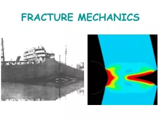
2. Stress based design vs Fracture Mechanics approach • Stress based criteria (like Von Mises) usually define the onset of “damage” initiation in the material • Once critical stress is reached, what happens? • In this case, a defect is now present (ie crack) • The key question is now: will it propagate? If yes, will it stop by itself or grow in an unstable manner. Stress concentrator: Critical stress is reached… A crack is formed… Will it extend further? If yes, will it propagate abruptly until catastrophic failure? Stress analysis Fracture mech.

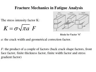
3. Propagation criteria of a crack Stress singularity • Crack propagation : stress intensity factor • Stress intensity factors KI, KII, KIII measure the intensity of stress singularity at crack tip. • “Stress intensity factor”: • Constants of the 1/sqrt(r) term in stress field at crack tip: • “Critical Stress intensity factor”: • Maximum K that a material can sustain, considered as a material property and indentified in standard fracture tests. Units: Pa/sqrt(m), symbol: KIcKIIcKIIIc • Crack propagation occurs if K > Kc with K=Kic+KIIc+KIIIc • In many materialy, propagation is mode I dominated: KI>KIc Assumed Crack extension dA Fracture test: measure force at failure and calculate KIc From analytical solutions or FE

4. Propagation criteria of a crack Potential energy: P0=U0-V0 • Crack propagation : an “energetic” process • Extend crack length: energy is used to create a new surface (break chemical bonds). • Driving “force”: internal strain energy stored in the system • “Energy release rate”: • Change in potential energy P (strain energy and work of forces) for an infinitesimal crack extension dA. Units: J/m2, Symbol: G • measure the crack “driving force” • “Critical Energy release rate”: • Energy required to create an additionnal crack surface. Is a material characteristic (but depends on the type of loading). Units: J/m2, symbol: Gc • Crack propagation occurs if G > Gc Assumed Crack extension dA Potential energy: P1= P0 –Er And Er = G*dA New crack surface dA: Dissipates Ed=Gc*dA

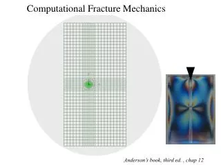
5. Computational Fracture Mechanics: Why? • Using numerical simulation method we can: • Apply Finite Element, Finite Volume/Difference, Boundary Element or Meshfree methods • To obtain approximations of displacement, force, stress and strain fields in arbitrary configuration. • And then? To apply fracture mechanics, we need: • to compute fracture mechanics parameters (SIF K, G) in 2D and 3D configurations; • to compute J integral in elastic-plastic analyses ; • to simulate crack growth (under general mixed-mode conditions); FE simulation of a compact tension fracture test

6. Overview of the different techniques • Calculation of K (linear elasticity): • Stress or displacement field matching (single / mixed mode) • Indirectly from G (Interaction integrals in mixed mode) • Calculation of G: • Finite difference of potential energy (linear, evtl. non linear) • Compliance method (linear) • Virtual Crack Closure Technique VCCT (linear, mixed mode) • J-integral (non-linear) • Simulate crack growth • to VCCT criterion, node release, remeshing or XFEM • Cohesive elements / interfaces (Damage mechanics)

7. Calculation of KI: stress matching • Idea: • compare FE stress field at crack tip with theory, • fit KI from the numerical stress value • In LEFM (for r  0): • Step 1: From FE: Extract stress field Syy at =0 (along crack direction) (eq 4.36a)

8. Calculation of KI: stress matching • Fitting method 1: Plot (as a function of r, for r  0) Fit region • Fit a line over the quasi constant region of the plot, identify KIeither as average value or as the interceptat r=0

9. Calculation of KI: stress matching • Fitting method 2: Plot as a function of • In theory the plot should be linear as: • Fit a line over the quasi linearregion of the plot, identify KIeither as the slope of the line Note : the same method can be applied to get Kii from shear component at theta=0

10. Calculation of KI: displacement matching • Idea: • compare FE crack displacement opening field with theory, • fit KI from the numerical displacement value • In LEFM (for r  0): • Step 1: From FE: Extract stress field Syy at =0 (along crack direction) (eq 4.40b) x m = shear modulus= For plane stress: For plane strain:

11. Calculation of KI: displacement matching • Fitting method 1: Plot (as a function of r=-x, for r  0) Fit region • Fit a line over the quasi constant region of the plot, identifyeither as the average value or as the interceptat r=0

12. Calculation of KI: displacement matching • Fitting method 1: Plot uy as a function • In theory, the plot should be linear as : • Fit a line over the quasi linearregion of the plot, the slopeis

13. Improving mesh convergence: singular elements • Evaluation of K from stress field requires very fine mesh. To better capture the 1/sqrt(r) stress singularity, one can use singular quadratic elements with shifted mid side nodes at ¼ of edge length (Barsoum,1976, IJNME, 10, 25; Henshell and Shaw, 1975, IJNME, 9, 495-507) • Using 8 node second order quadrangular elements, if we move the midside nodes at ¼ of edge, we make the Jacobian transformation of the element singular as 1/sqrt(r) along the element edges. • By collapsing all nodes of one edge (degenerate a quadrangle to a triangle), the 1/sqrt(r) singularity covers then the whole element. • Can be extended into 3D for 20 node hexahedrons

14. Computing K from G (and vice-versa) • For linear elastic isotropic materials, the following relations link G to K: m = shear modulus= • For Mode I in plane stress and plane strain, this simplifies to: • So knowing either K or G, the other can be determined directly. This can be extended to orthotropic material. For plane stress: For plane strain:

15. Calculation of G: Strain energy method • compare the strain energy of several FE models with different crack length, calculate the ERR as the derivative of potential energy  = U - F • For a linear elastic material: the potential energy F = PD = 2U thus  = U – F = - U with the strain energy • Compute ERR or as the slope of U(a) Different FE models for a0, a1, a2… a Equations are for a unit depth, if not the case, compute use U/b instead of U

16. Calculation of G: Compliance method • Idea (similar to experimental test data reduction !) • Calculate the compliance C(a)=D(a)/P(a) for different crack lengths a0, a1 (several FE models required) and fit it with an appropriate function • For a linear elastic material: the ERR can be obtained from the C(a) • Compute ERR where dC/da is obtained from the fitted curve (eq 3.41 & 3.43b) P, D Different FE models for a0, a1, a2… a

17. Calculation of G: J-integral method • Using the “J-Integral” approach (see course), it is possible to calculate the ERR G as G = J in linear elasticity. • If we know the displacement and stress field around the crack tip, we can compute J as a contour integral: • J-integral is path independent for all continuum materials. But G must be perpendicular to the interface if dissimilar materials are used. W=strain energy density u = displacement field s = stress field G = contour: ending and starting at crack surface

18. Calculation of G: J-integral method • J-integrals are usually computed from a volume/surface integral in FE, for example in Abaqus with q = virtual crack extension vector: • With on G and on C. Using divergence and equilibrium equations we can obtain:

19. J-integral in 3D: 3D effects J-integral can be extend in 3D by computing J on several “slices” of the model. However, there are notable 3D effects affecting crack propagation: in 3D, the external surface is free of normal stress, so in plane stress state For thick specimens, the center of the specimen is closer to plane strain state S22 on external surface Plane stress S22 on symmetry plane Plane strain => higher stresses

20. J-integral in 3D: 3D effects As a consequence, J-integral and G are not constant across the width. This will lead to a slightly curved crack front during propagation • Need to be careful about specimen size effects when characterizing G or K • In 2D FE simulation: use plane stress for very thin specimens, and plane strain for thick ones. G is max in the center => propagate earlier G is min on the side => propagate last

21. Comparison of methods • Results obtained on a relatively coarse 3D mesh to highlight which methods are less mesh sensitive Conclusion: K determination is more sensitive to mesh ! G calculation using compliance, J-integral or strain energy fit are the most reliable

22. J-integral in Abaqus Crack tip and extension direction • Can be calculated in elasticity / plasticity in 2D plane stress, plane strain, shell and 3D continuum elements. • Requires a purely quadrangular mesh in 2D and hexahedral mesh in 3D. • J-integral is evaluated on several “rings” of elements: need to check convergence with the # of ring) • Requires the definition of a “crack”: location of crack tip and crack extension direction Quadrangle mesh Crack plane Rings 1 & 2

23. J-Integral in Abaqus: application notes and demonstration • Create a linear elastic part, define an “independent” instance in Assembly module • Create a sharp crack: use partition tool to create a single edge cut, then in “interaction” module, use “Special->Crack->Assign seam” to define the crack plane (crack will be allowed to open) • In “Interaction”, use “Special->Crack->Create” to define crack tip and extension direction (can define singular elements here, see later for more info) • In “Step”: Define a “static” load step and a new history output for J-Integral. Choose domain = Contour integral, choose number of contours (~5 or more) and type of integral (J-integral). • Define loads and displacements as usual • Mesh the part using Quadrangle or Hexahedral elements, if possible quadratic. If possible use a refined mesh at crack tip (see demo). If singular elements are used, a radial mesh with sweep mesh generation is required. • Extract J-integral for each contour in Visualization, Create XY data -> History output. • !! UNITS: J = G = Energy / area. If using mm, N, MPa units => mJ / mm2 !!! • By default a 2D plane stress / plane strain model as a thickness of 1. See demo1.cae example file

24. Singular elements & meshing tips • To create a 1/sqrt(r) singular mesh: • In Interaction, edit crack definition and set “midside node” position to 0.25 (=1/4 of edge) & “collapsed element side, single node” • In Mesh: partition the domain to create a radial mesh pattern as show beside. Use any kind of mesh for the outer regions but use the “quad dominated, sweep” method for the inner most circle. Use quadratic elements to benefit from the singularity. • Refine the mesh around crack tip significantly.

25. J-integral Convergence vs # contours

26. Overview of the different techniques • Calculation of K (linear elasticity): • Stress or displacement field matching (single / mixed mode) • Indirectly from G (Interaction integrals in mixed mode) • Calculation of G: • Finite difference of potential energy (linear, evtl. non linear) • Compliance method (linear) • Virtual Crack Closure Technique VCCT (linear, mixed mode) • J-integral (non-linear) • Simulate crack growth • to VCCT criterion, node release, remeshing or XFEM • Cohesive elements / interfaces (Damage mechanics)

27. Virtual crack closure technique • VCCT is based on the calculation of the work done by elastic forces to close the crack tip, ie the work done to move the 1st node of the crack to its “closed” position • By decoupling normal and tangential displacement VCCT can be used to calculate mode I and II ERR in mixed mode case. • The work done to close the crack give the ERR: Wc= G*dA • Method 1: stiffness If the system is elastic: F=k d0 => Wc=2 x (1/2 k d02) => 2 step: compute d0, compute k F, d0 F, d0 L P, D Crack surface closed dA=L b: Ed=Gc*dA a

28. Virtual crack closure technique Step 1: external loading measure COD = 2*d0 • Method 1: stiffness If the system is elastic: F=k d0 => Wc=2 x (1/2 k d02) Step 1: • Apply loading conditions • FE solution => extract d0 Step 2: • Apply a closure force (dipole) F • FE solution => extract d1 • Compute k=F/(d0-d1) Compute work: Wc =2 x (1/2 k d02) and ERR:GI= Wc/dA=Wc/(L b) F, d1 d0 COD d0 F, d1 P, D P, D Step 2: perturbation F measure COD = 2*d1 a a

29. Virtual crack closure technique • Method 2: self similarity If the crack length extension da is small then the fields at crack tip can be considered self-similar (invariant with da) system is elastic. Only one step is then required for VCCT : (image srcAbaqus documentation) But with self similarity: Fj=Fi and di=di-1 Fi di-1 Fj di

30. VCCT: mixed mode GI, GII Mode mixity can be accounted for by decoupling the work into normal and tangential component: • GI is obtained from normal displacement and force dnandFn : GI=1/2 (Fn dn) / dA • GII from tangential displacement and force dt and Ft: GII=1/2 (Ft dt) / dA Fn dn Ft dt

31. Other Crack propagation criteria • Critical stress or opening displacement at a distance: Need to be calibrated on tests and are potentially mesh sensitive !! Not exactly a Fracture mechanics criterion, but can be related to ERR or K

32. Other Crack propagation criteria • Mixed mode crack propagation criteria: Combine GI,II,III in an expression Geq(GI,GII,GIII). Propagation if Geq>GeqCor Geq/GeqC>1 BK criterion: Power law : Need to be calibrated on mixed mode tests This requires a lot of work!!

33. Cohesive zone models (CZM) • Model energy dissipation in the process zone at crack tip by the work of dissipative forces. • CZM are based on damage mechanics and can model complex crack propagation in mixed mode, including fiber bridging. • Available either in the form of cohesive elements or cohesive contact formulations F, d Process zone: Plasticity, micro cracking… F, d CZM:Process zone= Cohesive forces

34. Cohesive zone models (CZM) • Basic ideas: • Discretize the fracture process zone and replace it by “springs” to represent crack tip forces (with a high stiffness K) • Model dissipation through evolution of damage D => K=(1-D) K0 • Evolve the damage variable D based on a “traction” – “crack opening” relationship F, d, F=sda F, d s Damage initiation (D=0) s=sc sc Damage propagation (D>0) Dissipated Energy Elastic unloading / reloading (D=cst) Total energy dissipated = G Final failure D=1 K0 d dc dmax

35. s Damage initiation (D=0) s=sc sc Damage propagation (D>0) K=(1-D) K0 Dissipated Energy Elastic unloading / reloading (D=cst, K=cst) K0 d K=(1-D) K0 dc dmax

36. s sc Elastic unloading / reloading (D=cst) Damage propagation (D>0) Final failure D=1 K0 d dmax Dissipated Energy

37. s sc Damage propagation (D>0) Final failure D=1 K0 d dmax Total Dissipated Energy = G = ½ scdmax

38. Cohesive zone models (CZM) How to define all those constants? Measure G from fracture tests and sc from a strength test Calculate dmax from G= ½ sc dmax K must be set sufficiently high (penalty stiffness) Recommendation: Estimate dc ~ dmax/ R with R ~ [10-100] Calculate K0 as K0 = sc / dc s Damage initiation (D=0) s=sc sc Damage propagation (D>0) Dissipated Energy G Final failure D=1 K0 d dc dmax

39. Cohesive zone models (CZM) • Example: crack propagation in an adhesive • G = 0.1 mJ/mm2 and sc = 10 MPa • dmax = 2 G/sc=0.02 mm • dc ~ dmax/ 10 => dc= 0.002 mm • K0 = sc / dc = 5000 N/mm DCB, plane strain, 25mm wide, 2x2.5 mm thick, 100mm length s d=5mm sc Tie constraints Adhesive layer: 0.2mm thick, 60mm long, Cohesive elements G K0 d dc dmax

40. How to model with CZ elements in Abaqus • In material properties: • define K in “Elastic” properties, type “Traction”; • Enter critical stress in “Damage for Traction separation Law” type QuadS for example • Add the option “Damage evolution”, based on Energy with Linear degradation etc.. . Enter G as critical ERR • Define a cohesive section and assign it to the “glue” layer: • type “Traction separation”, initial thickness = 1, out of plane thickness = 25 mm here. • In mesh: • Cohesive element MUST be generated as a single layer of elements using quad sweep (or hexa sweep) algorithms. The sweep direction will define the “normal” direction of the cohesive element! • Assign the type of element “Cohesive” (not by default) • In Step: • Set initial & max time increment to 0.05 (both) • Define a field output with the variable “SDEG” (= Damage D)

41. Fracture mechanics oriented design

42. Resources & help • Abaqus tutorials: • http://lmafsrv1.epfl.ch/CoursEF2012 • Abaqus Help: • http://lmafsrv1.epfl.ch:2080/v6.8 • See Analysis users manual, section 11.4 for fracture mechanics • Presentation and demo files: • http://lmafsrv1.epfl.ch/jcugnoni/Fracture • Computers with Abaqus 6.8: • 40 PC in CM1.103 and ~15 in CM1.110