Download
1 / 39
420 likes | 708 Vues
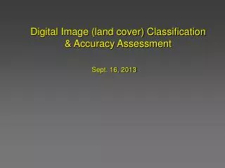
Digital Image (land cover) Classification & Accuracy Assessment. Sept. 16, 2013. Raster data model (digital image): 2-dimensional array of discrete values, displayed as an array of pixels representing earth surface features or attributes

E N D
Digital Image (land cover) Classification & Accuracy Assessment Sept. 16, 2013
Raster data model (digital image): 2-dimensional array of discrete values, displayed as an array of pixels representing earth surface features or attributes Range of discrete integer values varies depending on the data format (i.e. 8-bit ranges from 0-255) • continuous data: • discrete values represent quantitative variation in a continuously varying attribute or property • e.g. radiance recorded by an orbiting sensor • categorical or thematic data: • values represent qualitative categories or themes; actual pixel value has no inherent meaning • e.g. pixel values defining land cover classes - meaning is derived by associating a pixel value with a land cover type
2001 National Land Cover Database (NLCD) Continuous estimates of impervious surface cover Continuous estimates of canopy cover Categorical Land Cover
Digital image classification techniques use radiance • measured by a remote sensor in one or more wavebands • to sort pixels into information classes or themes. • end result is a thematic map • Digital image classification: • Sorting pixels into a finite number of classes or categories. • During visual image interpretation, you are continually sorting pixels into homogeneous areas that you associate with land cover features of interest. • You are essentially classifying image data using elements • of visual interpretation – tone (relative brightness), texture • (tonal variation), shape, size, pattern…)
Image (Land Cover) Classification Two Methods • Common classification procedures can be broken down into two broad categories: • unsupervised classification (Lab 3) • The computer separates features solely on their spectral properties – computer groups pixels into spectral classes • Analyst subsequently groups spectral classes into information classes (e.g., land cover types) • supervised classification(Lab 2) • Analyst uses prior knowledge of information classes to establish training sites, used to identify the spectral characteristics of those information classes • The computer then assigns each pixel into an information class according to its spectral characteristics
Spectral classes: Groups of pixels that are spectrally uniform or near-uniform -pixels that show similar brightness in the different wavebands for similar earth surface features. Information classes: Categories of interest (e.g. land cover classes such as forest, wetland, etc.) The objective of image classification is to match spectral classes to information classes.
Unsupervised Classification Iterative Self-Organizing Data Analysis Technique (ISODATA) Analyst sets the number of classes (e.g, 45), the number of iterations (e.g., 100) and the convergence threshold (e.g. .995). The # iterations and conv. threshold tells the ISODATA program when to quit. 1st iteration
Unsupervised Classification Iterative Self-Organizing Data Analysis Technique (ISODATA) 2nd iteration
Unsupervised Classification Iterative Self-Organizing Data Analysis Technique (ISODATA) 3rd iteration
Unsupervised Classification Iterative Self-Organizing Data Analysis Technique (ISODATA) ISODATA generating spectral classes (clusters) going into a statistical file – multivariate stats (mean, S.D., corr. matrix, co-var. matrix) in n-band space.
Supervised Classification The analyst identifies in the imagery representative and homogeneous samples of different surface cover types (information classes) of interest. These samples are referred to as training areas. The selection of training areas is based on the analyst's knowledge of the actual surface cover typesand location in the image/on ground. The analyst is "supervising" the categorization of a set of classes.
Supervised Classification 1. Training -identify homogeneous information classes and extraction of spectral signatures. Pick AOIs in Erdas Imagine. 2. Classification - automatic categorization of all pixels into information classes based on their spectral similarity to information classes.
255 Band 2 0 0 255 Band 1 Supervised Classification Computer groups pixels into information classes based on a “decision rule”.
255 Band 2 0 0 255 Band 1 Supervised Classification Supervised classification by the minimum distance to means decision rule
Group similar spectral classes into information classes (Imagine-recode) Multiple spectral classes grouped into each information class Single spectral class contains pixels ‘belonging to’ multiple information classes ‘Mixed coniferous/deciduous’ spectral class contains pixels belonging to the ‘Coniferous trees’ and ‘Deciduous trees’ information classes
Multiple spectral classes grouped into each information class Single spectral class contains pixels ‘belonging to’ multiple information classes So… the ‘Coniferous trees’ and ‘Deciduous trees’ information classes are not entirely spectrally separable – they are not differentiable based on their spectral properties alone
Remote sensors view earth surface features from above • A property of interest may not be directly ‘visible’ to the sensor • (e.g. properties measured beneath or within a forest canopy) - If a surface property does not directly affect spectral reflectance, it may be correlated with properties that do affect reflectance Many attributes of interest are indirectly distinguishable by their statistical association with attributes that directly affect spectral reflectance. Attributes that affect reflectance directly are easier to map. Forest composition is easier to map than forest structural attributes (stem diameter, height)
Hierarchical classification schemes allow users to organize data to a desired level of detail Detailed classes may be collapsed to improve map accuracy for certain applications
USGS Land Use / Land Cover Classification System Classification Level I Classification Level II Classification Level III • Urban or Built-Up Land • Agricultural Land • Rangeland • Forest Land • Water • Wetland • Barren Land • Tundra • Perennial Snow or Ice 11 Residential 12 Commercial, Services 13 Industrial 14 Transportation, Communications, Utilities 15 … 111 High-density residential 112 Low-density residential Moderate-resolution satellite imagery High-resolution satellite, high-altitude aerial imagery (<1:80,000 scale) Mid-altitude aerial imagery (1:20,000 to 1:80,000 scale)
Distribution of surface features of interest Vector map of surface features of interest Raster map of surface features of interest
Minimum Mapping Unit (MMU): The smallest area mapped as a discrete unit. For a raster map, MMU is determined by grouping adjacent pixel of like category, and then filtering to remove small groups.
Differences in MMU affect the spatial expression of patches on the mapped landscape. Small MMU: Greater heterogeneity; May be more difficult to identify patches or structure of importance Large MMU: Patches of interest may be artificially merged with neighboring patches
Classification Accuracy Assessment • “a classification is not complete until its accuracy has been assessed” • Why? • Crucial to know the quality of maps when using them to make resource decisions. • Increase map quality by identifying and correcting sources of error • In research applications, can often improve methods by comparing the accuracy resulting from use of various data, processing techniques, classification schemes, and interpreters
Quantitative Accuracy Assessment • Accuracy: the degree of correspondence between observation (e.g., classification) and reality (ground or surrogate of ground data) • Degree of correspondence is estimated from a set of sample locations • We usually judge accuracy against existing maps, aerial photos, or field checks - information used as reference and considered “truth”
Quantitative Accuracy Assessment 1) Specify sample design for selection of sample locations - Random, systematic, stratified random, clustered 2) Specify a sample size and gather reference data according to a specified protocol - Sample size may depend on size (area) of a class and desired precision with which map accuracy is estimated 3) Compare map labels to reference data and compile an error matrix describing distribution of error among classes 4) Compute various estimates of overall or class accuracy
CLASSIFIED IMAGE Generate a random sample of locations
REFERENCE DATA CLASSIFIED IMAGE From airphotos, field data, etc. Generate a random sample of locations
REFERENCE DATA CLASSIFIED IMAGE From airphotos, field data, etc. Generate a random sample of locations At each location, compare the map class with the reference class
Observed class membership: class membership derived from reference data, assumed correct (columns). • Number of correctly classified pixels shown along the major diagonal • Off-diagonals represent errors of omission and commission Accuracy Assessmentthe error matrix • Predicted class membership: mapped class membership derived from image classification procedure (rows). Observed class membership Predicted class membership
18 out of 43 pixels were committed to the corn category • corn category most confused with forest Accuracy Assessmentthe error matrix • Commission errors (errors of inclusion): Including an area in a category to which it does not truly belong Observed class membership Predicted class membership
7 out of 32 pixels were omitted from the corn category • corn category confused with forest, soybeans and other Accuracy Assessmentthe error matrix • Omission errors (errors of exclusion): Excluding an area from a category to which it does trulybelong Observed class membership Predicted class membership
Representations of map accuracy: overall accuracy (of the classification or map) user’s accuracy (1-commission error) producer’s accuracy (1-omission error) REFERENCE DATA CLASSIFIED IMAGE Accuracy Assessmentthe error matrix
Representations of map accuracy: overall accuracy (of the classification or map) user’s accuracy (commission error) producer’s accuracy (omission error) REFERENCE DATA CLASSIFIED IMAGE • Number of correctly classified pixels (sum of the major diagonal) • Divided by the number of total sampled pixels Accuracy Assessmentthe error matrix
Representations of map accuracy: user’s accuracy (1-commission error) REFERENCE DATA User’s accuracy forcorn category: CLASSIFIED IMAGE Accuracy Assessmentthe error matrix • The user is looking at a location on the map that says corn. • There is a 58% chance that the user would in fact find corn at that location in the field. • Divide the number of correctly classified pixels in each category by the number of pixels that were classified in that category (row total)
Representations of map accuracy: producer’s accuracy (1-omission error) REFERENCE DATA Producer’s accuracy forcorn category: CLASSIFIED IMAGE Accuracy Assessmentthe error matrix • At any given field location that is corn, there is a 78% chance that the analyst did in fact map that location as corn. • Divide the number of correctly classified pixels in each category by the number of reference pixels that were in that category (column total)
What does it mean that producer accuracy is so much higher than user accuracy?
Few errors of omission – Most corn on the ground is mapped Many errors of commission – A lot of other stuff is also mapped as corn. AREA mapped as cornfield is far greater than it should be.
Errors of omission are about as frequent as errors of commission. AREA mapped as sand is about what it should be, although there are considerable omission and commission errors.