Inventory
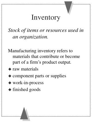
Inventory. Stock of items or resources used in an organization . Manufacturing inventory refers to materials that contribute or become part of a firm’s product output . raw materials component parts or supplies work-in-process finished goods. Purpose of Inventory.

Inventory
E N D
Presentation Transcript
Inventory Stock of items or resources used in an organization. Manufacturing inventory refers to materials that contribute or become part of a firm’s product output. • raw materials • component parts or supplies • work-in-process • finished goods
Purpose of Inventory • meet variation in product demand • provide safeguard for variation in raw material delivery • maintain independence of operations • allow flexibility in production scheduling • take advantage of quantity discounts
Inventory Costs • storage • handling • insurance and taxes • pilferage and breakage • obsolescence and depreciation • opportunity cost of capital • order processing • shipping and receiving • production setup and changeover • lost sales • backorders • lateness penalties
Inventory System Set of policies and controls that monitor levels of inventory (for all items).. . • determine what levels should be maintained • when stock should be replenished • how large an order should be • keep track of orders sent and received • reconcile records with physical inventory
Economic Order Quantity (EOQ) Model • Assumptions: • demand rate constant • instantaneous replenishment • price per item independent of order size • no backorders allowed • Questions: • When to order? • How much to order?
EOQ Model Inventory level Time Notation: D = demand rate per unit time (year) C = cost per unit item S = setup/order cost H = holding cost per unit item per unit time I = inventory holding percentage (H = IC) Q = quantity to be ordered
Total Cost (per unit time) = purchase cost + ordering cost + holding cost TC = DC + SD/Q + HQ/2 Best Q? or EOQ formula
Annual Product Costs,Based on Size of the Order TC (total cost) HQ/2 (holding cost) Cost DC (annual cost of items) SD/Q (ordering cost) Qopt Order quantity size (Q)
Number of units on hand Q Q Q Q R L L L Time Basic Fixed-Order Quantity Model with Lead Time Order when inventory drops to R = DL where L = lead time
inventory position on-hand inventory R L Inventory position =on-hand + on-order inventory
Buildup = Production rate minus usage rate (p-d) Production taking place No production; usage only Number of units on hand R Usage rate d Q L L EOQ with Usage • p = replenishment rate • d = demand rate
EOQ vs. JIT EOQ: order quantity set according to EOQ formula JIT: reduce inventory as much as possible Who is right? Who is wrong? What is the “right” order quantity? What is the “true” cost of inventory?
Inventory Pooling • What happens to the optimal order quantity when the demand rate doubles? Triples? Consequences? • Large supermarkets vs. mom-&-pop stores • “backup” agreements between stores
Global Supply/Distribution Chains • Decentralized System: • Centralized System: Retailers Factory Depot Factory Retailers
Inventory Management-Single Period Model • order placed (and delivered) before demand is known • unmet demand is lost • unsold inventory at the end of the period is discard (or salvaged at lower value) How much to order? Newsboy Model
Marginal Profit = MP = profit resulting from last unit sold Marginal Loss = ML = loss from last unit unsold Newsvendor Model Stock one unit if ... MP Pr(D > 0) > ML Pr(D < 0) Stock 2 units if ... Stock 1 Stock 2 D = 0 D = 1 D = 2 D = 3 D = 4
Newsvendor Model 0 keep order size at 1 -ML 1 more unsold order 2 instead of 1 MP 1 fewer lost sale Additional Benefit Order 2 if Pr(D<1) (-ML) + Pr(D>1) MP > 0 or Pr(D<1) (-ML) + [1-Pr(D<1)] MP > 0 or Pr(D<1) < MP ML + MP Increase order to n+1 if Prob(Demand > n) < MP ML + MP
EXAMPLE / Salvage Value A product is priced to sell at $100 per unit, and its cost is constant at $70 per unit. Each unsold unit has a salvage value of $30. Demand is expected to range between 35 and 40 units for the period: 35 units definitely can be sold and no units over 40 will be sold. The demand probabilities and the associated cumulative probability distribution (P) for this situation are shown below. The marginal profit if a unit is sold is the selling price less the cost, or MP = $100 - $70 = $30. The marginal loss incurred if the unit is not sold is the cost of the unit less the salvage value, or ML = $70 - $30 = $40. How many units should be ordered? SOLUTION The optimal probability of the last unit being sold is
According to the cumulative probability table (the last column in table below, 37 units should be stocked. The net benefit from stocking the 37th unit is the expected marginal profit minus the expected marginal loss. EXHIBIT 14.12 Demand and Cumulative Probabilities (p) CPn Number of Units Probability of Demanded This Demand 35 0.10 1 to 35 0.10 36 0.15 36 0.25 37 0.25 37 0.50 38 0.25 38 0.75 39 0.15 39 0.90 40 0.10 40 1.00 41 0 41 or more 1.00
EXHIBIT 14.13 Marginal Inventory Analysis for Units Having Salvage Value (N) (p) (P) (MP) (ML) Units of Probability CPn Expected Marginal Expected Marginal Demand of Demand Profit of n-th Unit Loss of n-th Unit (Net) (100-70)(1- CPn-1) (70-30)CPn-1 (MP)-(ML) 35 0.10 0.10 $30 $0 $30.00 36 0.15 0.25 27 4 23.00 37 0.25 0.50 22.50 10 12.50 38 0.25 0.75 15 20 (5.00) 39 0.15 0.90 7.50 30 (22.50) 40 0.10 1.00 3 36 (33.00) 41 0 1.00 (40.00) Note: Expected marginal profit is the selling price of $100 less the unit cost of $70 times the probability the unit will be sold. Expected marginal loss is the unit cost of $70 less the salvage value of $30 times the probability the unit will not be sold. Net = (MP)(1 - CPn-1 ) - (ML) CPn-1 = (1 - 0.25)($100 - $70) - (0.75) ($70 - $30) = $22.50 - $10.00 = $12.50 For the sake of illustration, Exhibit 14.13 shows all possible decisions. From the last column, we can confirm that the optimum decision is 37 units.
y Newsvendor Model-Demand Distribution Continuous Order y such that Prob(Demand < y) = MP . ML+MP
Summary • Uses and Costs of inventory • EOQ Model • lead time OK • non-instantaneous replenishment OK • constant demand rate • no backorders • Demand Stochastic? • Newsvendor model