Download
1 / 61
630 likes | 792 Vues
Modeling Heat Flow in a Thermos. Michael A. Karls James E. Schershel Ball State University. The Coffee Cup Problem. Freshly poured coffee has a temperature of 80 o C. Assume that the room temperature is a constant 20 o C, and that after two minutes, the coffee has cooled to 70 o C .

E N D
Modeling Heat Flow in a Thermos Michael A. Karls James E. Schershel Ball State University
The Coffee Cup Problem • Freshly poured coffee has a temperature of 80 oC. • Assume that the room temperature is a constant 20 oC, and that after two minutes, the coffee has cooled to 70 oC . • Find a model for the temperature of the coffee at any time after the coffee is first poured.
Newton’s Law of Cooling • Newton's law of cooling*: The rate of temperature change of an object is proportional to the difference in temperature between the object and its surroundings. • Newton’s law of cooling can be used to model a cooling cup of coffee! • *Newton experimentally observed that the rate of loss of temperature of a hot body is proportional to the temperature itself, but it was Fourier who actually wrote down an equation to describe this process of heat transfer.
The Coffee Cup Model • Using Newton's law of cooling, a model for a cooling cup of coffee is given by the following initial value problem for t 2 (-1,1): where • k>0 is a proportionality constant that describes the rate at which the coffee cools, • T is the surrounding temperature, • T0 is the initial temperature of the coffee, • u(t) is the temperature of the coffee at any time t. • The solution to (1), (2) is:
Verifying the Coffee Cup Model Experimentally • Texas Instruments (TI) has developed an inexpensive calculator-sized data collection interface, known as a Calculator-Based Laboratory (CBL). • The CBL provides a link between a TI calculator and sensors that are used to collect data. • Some of the sensors available: • pH • Temperature • Pressure • Force • Motion • Using a CBL with a temperature probe, a TI-85 calculator, and a program available from TI’s website (http://education.ti.com/) , temperature data can be collected, plotted, and compared to the solution in (3).
A Modified Coffee Cup Problem • What if we wish to know the temperature at any position within the cup of coffee at any particular time? • One way to approach this problem: Think of the water in the cup as a cylinder of heat conducting material that is insulated on the side, top, and bottom. • Instead of a cup full of coffee, we can think of a thermos full of coffee!
The Thermos Problem • A thermos is filled with hot coffee at an initial temperature of 80 oC. • Assume that the room temperature is 20 oC and the top of the thermos is left open. • Find a model for the temperature of the coffee at any position in the thermos and at any time after the coffee is first poured.
Heat Flow in a Rod • Joseph Fourier made an extensive study of heat flow in objects such as a long rod of conducting material with an insulated lateral surface. • Although we are not considering a solid, we can try to use the same ideas to model the temperature in a cylindrical column of hot coffee! • Our goal is to find a model for the temperature of the coffee in a thermos at any time and at any position and show that this model agrees with actual data. • Instead of hot coffee, we’ll look at ice-cold water.
The Thermos Model • Assume we have a thermos full of ice-cold water, open at the top. • Since the water is ice-cold, we’ll assume: • There is no internal convection. • The contribution of heat from radiation is negligible. • There is no evaporative cooling at the top. • Think of the ice-cold water as a cylinder of conducting material that is insulated at the bottom and on the side. • Heat is transferred by convection at the top surface of the water. • Assume that at any time the temperature will be the same at any point of a cross-sectional slice of water.
Let u(y,t) be the temperature at any cross-sectional slice of the water, for 0 · y · a; t ¸ 0. Let y = 0 and y = a correspond to the bottom and top of the thermos, respectively. Assume the air surrounding the thermos is at constant temperature T0. Suppose the initial temperature distribution is given some sectionally smooth function f(y). By sectionally smooth, we mean f'(y) exists and is continuous on [0,a], except possibly at a finite number of jumps or removable discontinuities. The Thermos Model (cont.) y = 0 y = a
The Thermos Model (cont.) • This simple system can then be modeled by the following initial value-boundary value problem for 0<y<a, t>0: • Equation (4) is known as the one-dimensional heat equation and , c, , and h are the density, specific heat, thermal conductivity, and convection coefficient, respectively.
Recall Fourier's law of heat conduction where q(y,t) is the heat flow rate. Using (8), we see that boundary condition (5) indicates that there is no heat flow through the bottom of the thermos. Similarly, (8) shows that boundary condition (6) describes the interaction of the top of the water with the air via Newton's law of cooling. The known initial temperature distribution is given by (7). The Thermos Model (cont.)
The Thermos Model (cont.) • Using the technique of separation of variables or Fourier’s Method, the solution to (4)-(7) is found to be: where n is the unique solution to in the interval • The coefficients Bn are given by:
Now that we have a model for our thermos, we collect temperature data and test our model experimentally. The following materials are required: Four TI-85 calculators with temperature collection software Four CBLs with temperature probes One thermos Two twist ties One rubber band Ice Water Ruler Freezer Verifying the Thermos Model Experimentally
Experimental Procedure • The experimental procedure is as follows: • Measure the depth of the interior of the thermos. • Use the two twist-ties to connect three of the temperature probe cables together, with the probes arranged so that the distance between each probe is half of the depth of thermos. • Place the probes in the freezer. • Fill the thermos with ice water and allow it to sit for roughly two hours to pre-chill. • Then remove the ice from the thermos and top-off the thermos with ice-cold water.
Experimental Procedure (cont.) • Insert the three temperature probes that are twist-tied together into the thermos and use the rubber band to keep the probes at the proper heights: one at the bottom, one in the middle, and one at the top, just below the surface of the water. Use the fourth temperature probe to record the ambient room temperature. • Use the TI-85 calculators and the CBLs to record the temperature data. • Collect temperature data once every 120 sec for 4 hr.
Assigning Values to Coefficients in Our Model • To compare our model to the experimental data, we need to specify the parameters in the model. • Length of the thermos: a = 0.28 m • Ambient room temperature: T0 = 21 oC. • Density of water: = 1000 kg/m3 • Specific heat of water: c = 4186 J/(kg oC) • Thermal conductivity of water: = 0.602784 J/(m s oC) • Convection coefficient is h = 83.72 J/(m 2 s oC). • The choice for convection coefficient is a guess based on convection coefficients found in the paper “The virtual cook: Modeling heat transfer in the kitchen,” Physics Today 52 (11), pp. 30—36 (1999).
Initial Temperature Distribution • We also need to specify an initial temperature distribution function f(y). • If the thermos were well-shaken, we would expect that the temperature would initially be uniform. • Experimentally we find: • The temperature readings initially decrease slightly, then rise. • The top of the thermos has a higher initial temperature than the middle and bottom.
Initial Temperature Distribution (cont.) • To take this temperature difference into account, we use a piecewise linear function for f(y). • f(y) is constructed from the points (0,Tb) , (a/2,Tm) , and (a,Ta) , where Tb, Tm , and Ta are the measured initial temperatures at the bottom (y = 0), middle ( y = a/2), and top ( y = a), respectively.
We now use (10) and (11) to find the values of n numerically. These values of n and the initial temperature distribution f(y) can then be substituted into (12) to find the coefficients, Bn, for our model. Graphically comparing the nth partial sum of (9) at t = 0 to the initial temperature distribution f(y) , thirty terms in (9) appear to be enough for our model. Determining the Number of Terms in Our Model
Model vs. Experimental Results • Unfortunately, as we see in Fig. 1, the model doesn't match the experimental results very well. • How far are we off? One measure of the error is the mean of the sum of the squares for error (MSSE) which is the average of the sum of the squares of the differences between the measured and model data values • MSSE for this model: • Top(): 33.7 (oC)2, • Middle(): 0.534 (oC)2, • Bottom(): 0.930 (oC)2. Figure 1 Model: _________ Actual: …………….
Maybe the problem with our model is our choice of the constant h, which was chosen fairly arbitrarily. With the choice of h=920.92 J/(m2 s oC), found by finding the best fit with integer multiples of our initial guess of h, we obtain the results shown in Fig. 2 after recomputing the values of n and Bn. Although the model is significantly closer to the experimental results for the temperature at the top of the thermos, the model is still off by about the same amount for the middle and bottom of the thermos. MSSE for this model: Top(): 1.11 (oC)2, Middle(): 0.468 (oC)2, Bottom(): 0.929 (oC)2. Model with New Constants vs. Experimental Results Figure 2 Model: _________ Actual: …………….
Modified Experimental Procedure • Perhaps our assumption that convection plays no significant role is incorrect. • To reduce the contribution of this pathway for heat flow, we make the following modification to our experimental procedure and pack the thermos with cotton balls to reduce convection currents. • The following additional materials are required for the revised experimental procedure: • One bag of 100 cotton balls • One pencil
Modified Experimental Procedure (cont.) • The modified experimental procedure is as follows: • Measure the depth of the interior of the thermos. • Use the two twist-ties to connect three of the temperature probe cables together, with the probes arranged so that the distance between each probe is half of the depth of thermos. • Place the probes and pencil in the freezer. • Fill the thermos with cotton balls, remove the cotton balls and place them in the freezer. • Fill the thermos with ice water and allow it to sit for roughly two hours to pre-chill. • Remove the ice from the thermos and top-off the thermos with ice-cold water.
Modified Experimental Procedure (cont.) • Take the cotton balls from the freezer and add the cotton balls one-by-one to the thermos. Use the chilled pencil to poke them below the waterline. • Insert the three temperature probes that are twist-tied together into the thermos and use the rubber band to keep the probes at the proper heights: one at the bottom, one in the middle, and one at the top, just below the surface of the water. Use the fourth temperature probe to record the ambient room temperature. • Use the TI-85 calculators and the CBLs to record the temperature data.
Modified Experimental Procedure (cont.) • We can now re-test our model using the modified experimental procedure. The same values of a, , and c are used. • The ambient temperature for this data set is slightly higher, so we take T0 = 24 oC. • Because the cotton, probe leads, and convection could affect the apparent value of and our choice for h was really just a guess, we choose and h so that the model matches the data as closely as possible graphically. • By tripling our initial choice of and taking multiples of an initial guess for h =41.86 J/(m2 s oC), we find that =1.80835 J/(m s oC) and h=1004.64 J/(m2 s oC) work well.
If we construct a new piecewise linear f(y) and compute n and Bn for our new model data, we obtain the results shown in Fig. 3 with thirty terms in the sum for u(y,t). Visually, the model seems to be closer to experimental results, but the bottom and middle model values are still off. MSSE for this model: Top(): 0.396 (oC)2, Middle(): 0.576 (oC)2, Bottom:() 0.487 (oC)2. Model With New Constants vs. Modified Experimental Results Figure 3 Model: _________ Actual: …………….
A Final Modification to Our Model • As a final modification of our model, suppose that we had started with a different initial temperature distribution, say f(y)=A eB y+C. • This form of f(y) is chosen to model the rapid rise in initial temperature near the top of the thermos. • To take into account the fact that the temperature readings initially decrease slightly, then rise, we will use the points (0, Tmin,b), (a/2,Tmin,m), and (a,Tmin,a), where Tmin,b, Tmin,m, and Tmin,a are the minimum temperature readings recorded at these positions.
To find the unknown constants A, B, and C, we solve the system of equations: A Final Modification to Our Model (cont.)
Modified Model vs. Modified Experimental Results • As before, we compute n and Bn using the same and h as in the previous model. Fig. 4 shows our results. • Of the models we have tried, this one provides the best visual fit to the experimental data. • MSSE for this model: • Top(): 0.142 (oC)2, • Middle(): 0.0664 (oC)2, • Bottom(): 0.0449 (oC)2. Figure 4 Model: _________ Actual: …………….
As a final test of our model, we'll use it to answer the question: How long does the thermos keep things cold? To do so, we look at the average value of the temperature of the water as a function of time, which is given by the integral Computing this integral numerically, as we see in Fig. 5, the model predicts that the temperature of the thermos will warm up to 15 oC in about 1.42 days. Experimentally, the thermos warms up to about 16 oC in a day and a half. A Final Test of Our Model Figure 5 Model Ave Temperature: _________ “Cold” Temp < 15 oC: _________
Conclusions and Further Questions • Using Fourier's model for heat conduction, we have developed a simple model for the temperature of ice-cold water in a thermos at any position and any time. • Based on experimental data, we found that a modified version of our original model agrees with our measured data. • One question that arises is why does our last choice of the initial temperature distribution work so well?
Conclusions and Further Questions (cont.) • The main heat transfer mechanism in the thermos is some combination of conduction and convection. • In practice, when modeling heat transfer due to conduction or convection, it turns out that Newton's law of cooling can be used to describe the heat flow rate. • Therefore, if we assume that for small t, the temperature in the thermos doesn't change with time, a natural choice for the initial heat flow rate at any point in the thermos would be:
Conclusions and Further Questions (cont.) where Ts is the unknown temperature at the surface of the ice-water and ĥ is a proportionality constant. • From Fourier's law of heat conduction, we see that for 0<y<a, which has the general solution where A, Ts, and ĥ/ are unknown constants. Equation (23) is exactly the form of our final choice of f(y)!!
Conclusions and Further Questions (cont.) • This experiment can be safely performed by students in a classroom setting for the small cost of four calculators, four CBLs, and a decent thermos (such as our choice of a Stanley heavy duty thermos). • Note that the constants h, k, and T0 may need to be adjusted to match a different experimental environment.
Conclusions and Further Questions (cont.) • In addition to the experiment we have outlined, other questions such as the following could be addressed. • How does adjusting the constants h and k affect the discrepancy between the model and the actual data? • Instead of choosing h and k by trial and error, are there mathematical methods that could be used to minimize the discrepancy? • What happens if a liquid with different chemical composition than water, such as cola or lemonade, is put in the thermos? Can h and k still be chosen to match the model to the measured data? • How well does this model work with hot coffee in the thermos instead of ice-cold water? • In a model with a hot liquid, are there any other factors that need to be considered, such as heat lost due to evaporation?
Resources • The MacTutor History of Mathematics archive: http://www-history.mcs.st-andrews.ac.uk/index.html • Texas Instruments Educational Resources: http://education.ti.com/ • “Modeling Heat Flow in a Thermos”, Am. J. Phys. 71 (7), July 2003
To solve (4)-(7), we first find the steady-state solution v(y), where v(y) is the limit of u(y,t) as t ! 1. Intuitively, we expect that after a long time, the water in the thermos should warm to room temperature and become independent of time. Letting t !1 in (4)-(7), we find that for 0<y<a, v(y) satisfies: IVBVP for Thermos Solution of the IVBVP
The Steady-State Problem • The unique solution to (24)-(26) is v(y) ´ T0. • Because u(t,y) ! v(y) as t !1, if we let w(y,t) = u(y,t) – v(y), it follows that w(y,t) ! 0 as t !1. • For this reason, we call w(y,t) the transient solution of (1)-(4).
The Transient Problem • Substituting u(y,t)=w(y,t)+v(y) into (1)-(4), we obtain the transient problem for 0<y<a, t>0: where g(y) ´ f(y)-T0. • To solve (27)-(30), we use separation of variables, or Fourier’s method. With the assumption that w(y,t) = (y)T(t), (27)-(29) become:
Separation of Variables • Rearranging (31), we see that for all 0<y<a and for all t>0, • For (35) to hold, both sides must have some common constant value.
From (32) and (33) we obtain boundary conditions in terms of the product of (y) and T(t). Equation (32) implies that either T(t)=0 for all t or '(0)=0. Because we want a non-trivial transient solution, we choose Similarly, (33) implies that either T(t)=0 for all t, or Separation of Variables (cont.)
Separation of Variables (cont.) • Setting both sides of (35) equal to common constant A0, we find that (y) and T(t) satisfy • The solutions to (39) are of the form where is some real constant. • The solution to (38) depends on the choice of constant A0 and the boundary conditions (36), ’(0)=0, and (37)
Separation of Variables (cont.) • To have nontrivial transient solutions that decay to zero as t !1, A0 must be negative. • For convenience, we write A0=-2, with >0. Then (38) has solutions of the form: • Since (36) implies ’(0) = 0, c2 = 0 must hold. • From the other boundary condition, (37), we see that which means that either c1 = 0, leading to trivial w(y,t) ´ 0, or must satisfy:
Separation of Variables (cont.) • One can show that there are infinitely many solutions to (43), with one in each interval: where n is a positive integer.
Separation of Variables (cont.) • Thus to each positive integer n = 1, 2, 3, …, there corresponds a solution to (27)-(29): with n satisfying:
Separation of Variables (cont.) • Also, for each positive integer n, there is a corresponding solution to (39) of the form • It follows that for each positive integer n, we have a solution to (27)-(29) of the form
Separation of Variables (cont.) • Note that the boundary value problem is a special case of a more general problem known as a regular Stürm-Liouville problem. • When a function (y) solves this type of problem for a certain 2, we call an eigenfunction with eigenvalue2. • The eigenfunctions and eigenvalues for this problem satisfy the orthogonality condition: