Download
1 / 54
540 likes | 658 Vues
Explore statistical learning, function optimization, neural networks, SVMs, and Kernel functions for classification and regression. Learn about maximizing geometric margins, kernel tricks, and feature mappings in SVMs for efficient learning strategies.

E N D
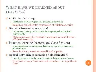
What have we learned about learning? • Statistical learning • Mathematically rigorous, general approach • Requires probabilistic expression of likelihood, prior • Decision trees (classification) • Learning concepts that can be expressed as logical statements • Statement must be relatively compact for small trees, efficient learning • Function learning (regression / classification) • Optimization to minimize fitting error over function parameters • Function class must be established a priori • Neural networks (regression / classification) • Can tune arbitrarily sophisticated hypothesis classes • Unintuitive map from network structure => hypothesis class
Motivation: Feature Mappings • Given attributes x, learn in the space of features f(x) • E.g., parity, FACE(card), RED(card) • Hope CONCEPT is easier to learn in feature space
Example x2 x1
Example • Choose f1=x12, f2=x22, f3=2 x1x2 x2 f3 f2 f1 x1
VC dimension • In an N dimensional feature space, there exists a perfect linear separator for n <= N+1 examples no matter how they are labeled ? + - + - + - + + - -
SVM Intuition • Find “best” linear classifier in feature space • Hope to generalize well
Linear classifiers • Plane equation: 0 = x1θ1+ x2θ2 + … + xnθn + b • If x1θ1 + x2θ2 + … + xnθn + b > 0, positive example • If x1θ1 + x2θ2 + … + xnθn + b < 0, negative example Separating plane
Linear classifiers • Plane equation: 0 = x1θ1+ x2θ2 + … + xnθn + b • If x1θ1 + x2θ2 + … + xnθn + b > 0, positive example • If x1θ1 + x2θ2 + … + xnθn + b < 0, negative example Separating plane (θ1,θ2)
Linear classifiers • Plane equation: x1θ1+ x2θ2 + … + xnθn + b = 0 • C = Sign(x1θ1 + x2θ2 + … + xnθn + b) • If C=1, positive example, if C= -1, negative example Separating plane (θ1,θ2) (-bθ1, -bθ2)
Linear classifiers • Let w = (θ1,θ2,…,θn) (vector notation) • Special case: ||w|| = 1 • b is the offset from the origin The hypothesis space is the set of all (w,b), ||w||=1 Separating plane w b
Linear classifiers • Plane equation: 0 = wTx + b • If wTx+ b > 0, positive example • If wTx+ b < 0, negative example
SVM: Maximum Margin Classification • Find linear classifier that maximizes the margin between positive and negative examples Margin
Margin • The farther away from the boundary we are, the more “confident” the classification Margin Not as confident Very confident
Geometric Margin • The farther away from the boundary we are, the more “confident” the classification Margin Distance of example to the boundary is its geometric margin
Geometric Margin • Let yi = -1 or 1 • Boundary wTx + b = 0, =1 • Geometric margin is y(i)(wTx(i)+ b) SVMs try to optimize the minimum margin over all examples Margin Distance of example to the boundary is its geometric margin
Maximizing Geometric Margin maxw,b,mm Subject to the constraintsm y(i)(wTx(i)+ b),=1 Margin Distance of example to the boundary is its geometric margin
Maximizing Geometric Margin minw,b Subject to the constraints1 y(i)(wTx(i)+ b) Margin Distance of example to the boundary is its geometric margin
Key Insights • The optimal classification boundary is defined by just a few (d+1) points: support vectors Margin
Using “Magic” (Lagrangian duality, Karush-Kuhn-Tucker conditions)… • Can find an optimal classification boundary w = Siai y(i) x(i) • Only a few ai’s at the SVs are nonzero (n+1 of them) • … so the classificationwTx= Siai y(i) x(i)Txcan be evaluated quickly
The Kernel Trick • Classification can be written in terms of(x(i)T x)… so what? • Replaceinner product (aTb) with a kernel function K(a,b) • K(a,b)= f(a)Tf(b) for some feature mapping f(x) • Can implicitly compute a feature mapping to a high dimensional space, without having to construct the features!
Kernel Functions • Can implicitly compute a feature mapping to a high dimensional space, without having to construct the features! • Example: K(a,b) = (aTb)2 • (a1b1 + a2b2)2= a12b12 + 2a1b1a2b2 + a22b22= [a12, a22 , 2a1a2]T[b12, b22 , 2b1b2] • An implicit mapping to feature space of dimension 3 (for n attributes, dimension n(n+1)/2)
Types of Kernel • Polynomial K(a,b) = (aTb+1)d • Gaussian K(a,b) = exp(-||a-b||2/s2) • Sigmoid, etc… • Decision boundariesin feature space maybe highly curved inoriginal space!
Kernel Functions • Feature spaces: • Polynomial: Feature space is exponential in d • Gaussian: Feature space is infinite dimensional • N data points are (almost) always linearly separable in a feature space of dimension N-1 • => Increase feature space dimensionality until a good fit is achieved
Nonseparable Data • Cannot achieve perfect accuracy with noisy data • Regularization parameter: • Tolerate some errors, cost of error determined by some parameter C • Higher C: more support vectors, lower error • Lower C: fewer support vectors, higher error
Soft Geometric Margin Regularization parameter minw,b,e Subject to the constraints1-ei y(i)(wTx(i)+ b)0 ei Slack variables: nonzero only for misclassified examples
Comments • SVMs often have very good performance • E.g., digit classification, face recognition, etc • Still need parametertweaking • Kernel type • Kernel parameters • Regularization weight • Fast optimization for medium datasets (~100k) • Off-the-shelf libraries • SVMlight
So far, most of our learning techniques represent the target concept as a model with unknown parameters, which are fitted to the training set • Bayes nets • Least squares regression • Neural networks • [Fixed hypothesis classes] • By contrast, nonparametric models use the training set itself to represent the concept • E.g., support vectors in SVMs
- - + - + - - - - + + + + - - + + + + - - - + + Example: Table lookup • Values of concept f(x) given on training set D = {(xi,f(xi)) for i=1,…,N} Example space X Training set D
- - + - + - - - - + + + + - - + + + + - - - + + Example: Table lookup • Values of concept f(x) given on training set D = {(xi,f(xi)) for i=1,…,N} • On a new example x, a nonparametric hypothesis h might return • The cached value of f(x), if x is in D • FALSE otherwise Example space X Training set D A pretty bad learner, because you are unlikely to see the same exact situation twice!
Nearest-Neighbors Models • Suppose we have a distance metricd(x,x’) between examples • A nearest-neighbors model classifies a point x by: • Find the closest point xi in the training set • Return the label f(xi) X - + + - + - + - - + Training set D - +
Nearest Neighbors • NN extends the classification value at each example to its Voronoi cell • Idea: classification boundary is spatially coherent (we hope) Voronoi diagram in a 2D space
Distance metrics • d(x,x’) measures how “far” two examples are from one another, and must satisfy: • d(x,x) = 0 • d(x,x’) ≥ 0 • d(x,x’) = d(x’,x) • Common metrics • Euclidean distance (if dimensions are in same units) • Manhattan distance (different units) • Axes should be weighted to account for spread • d(x,x’) = αh|height-height’| + αw|weight-weight’| • Some metrics also account for correlation between axes (e.g., Mahalanobis distance)
Properties of NN • Let: • N = |D| (size of training set) • d = dimensionality of data • Without noise, performance improves as N grows • k-nearest neighbors helps handle overfitting on noisy data • Consider label of k nearest neighbors, take majority vote • Curse of dimensionality • As d grows, nearest neighbors become pretty far away!
Curse of Dimensionality • Suppose X is a hypercube of dimension d, width 1 on all axes • Say an example is “close” to the query point if difference on every axis is < 0.25 • What fraction of X are “close” to the query point? ? ? d=2 d=3 d=10 d=20 0.52 = 0.25 0.53 = 0.125 0.510= 0.00098 0.520= 9.5x10⁻⁷
Computational Properties of K-NN • Training time is nil • Naïve k-NN: O(N) time to make a prediction • Special data structures can make this faster • k-d trees • Locality sensitive hashing • … but are ultimately worthwhile only when d is small, N is very large, or we are willing to approximate See R&N
Nonparametric Regression • Back to the regression setting • f is not 0 or 1, but rather a real-valued function f(x) x
Nonparametric Regression • Linear least squares underfits • Quadratic, cubic least squares don’t extrapolate well Cubic f(x) Linear Quadratic x
Nonparametric Regression • “Let the data speak for themselves” • 1st idea: connect-the-dots f(x) x
Nonparametric Regression • 2nd idea: k-nearest neighbor average f(x) x
Locally-weighted Averaging • 3rd idea: smoothed average that allows the influence of an example to drop off smoothly as you move farther away • Kernel function K(d(x,x’)) K(d) d=0 d=dmax d
Locally-weighted averaging • Idea: weight example i bywi(x)= K(d(x,xi)) / [Σj K(d(x,xj))](weights sum to 1) • Smoothed h(x) = Σi f(xi) wi(x) xi f(x) wi(x) x
Locally-weighted averaging • Idea: weight example i bywi(x)= K(d(x,xi)) / [Σj K(d(x,xj))](weights sum to 1) • Smoothed h(x) = Σi f(xi) wi(x) xi f(x) wi(x) x
What kernel function? • Maximum at d=0, asymptotically decay to 0 • Gaussian, triangular, quadratic Kparabolic(d) Kgaussian(d) Ktriangular(d) d d=0 0 dmax
Choosing kernel width • Too wide: data smoothed out • Too narrow: sensitive to noise xi f(x) wi(x) x
Choosing kernel width • Too wide: data smoothed out • Too narrow: sensitive to noise xi f(x) wi(x) x
Choosing kernel width • Too wide: data smoothed out • Too narrow: sensitive to noise xi f(x) wi(x) x
Extensions • Locally weighted averaging extrapolates to a constant • Locally weighted linear regression extrapolates a rising/decreasing trend • Both techniques can give statistically valid confidence intervals on predictions • Because of the curse of dimensionality, all such techniques require low d or large N