Exponential Functions Logarithmic Functions Compound Interest

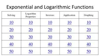
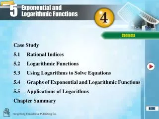
1. 5 • Exponential Functions • Logarithmic Functions • Compound Interest • Differentiation of Exponential Functions • Exponential Functions as Mathematical Models Exponential and Logarithmic Functions

2. 5.1 Exponential Functions

3. Exponential Function • The function defined by is called an exponential function with baseb and exponentx. • The domain of f is the set of all real numbers.

4. Example • The exponential function with base2 is the function with domain(–, ). • Find the values of f(x) for selected values of x follow:

5. Example • The exponential function with base2 is the function with domain(–, ). • Find the values of f(x) for selected values of x follow:

6. Laws of Exponents • Let a and b be positive numbers and let x and y be real numbers. Then,

7. Examples • Let f(x) = 22x – 1. Find the value of x for which f(x) = 16. Solution • We want to solve the equation 22x – 1= 16 = 24 • But this equation holds if and only if 2x – 1 = 4 giving x = . Example 2, page 331

8. Examples • Sketch the graph of the exponential function f(x) = 2x. Solution • First, recall that the domain of this function is the set of real numbers. • Next, putting x = 0 gives y = 20 = 1, which is the y-intercept. (There is no x-intercept, since there is no value of x for which y = 0) Example 3, page 331

9. Examples • Sketch the graph of the exponential function f(x) = 2x. Solution • Now, consider a few values for x: • Note that 2xapproaches zero as xdecreases without bound: • There is a horizontal asymptote at y = 0. • Furthermore, 2xincreases without bound when xincreases without bound. • Thus, the range of f is the interval(0, ). Example 3, page 331

10. Examples • Sketch the graph of the exponential function f(x) = 2x. Solution • Finally, sketch the graph: y 4 2 f(x) = 2x x –2 2 Example 3, page 331

11. Examples • Sketch the graph of the exponential function f(x) = (1/2)x. Solution • First, recall again that the domain of this function is the set of real numbers. • Next, putting x = 0 gives y = (1/2)0 = 1, which is the y-intercept. (There is no x-intercept, since there is no value of x for which y = 0) Example 4, page 332

12. Examples • Sketch the graph of the exponential function f(x) = (1/2)x. Solution • Now, consider a few values for x: • Note that (1/2)xincreases without bound when xdecreases without bound. • Furthermore, (1/2)xapproaches zero as xincreases without bound: there is a horizontal asymptote at y = 0. • As before, the range of f is the interval(0, ). Example 4, page 332

13. Examples • Sketch the graph of the exponential function f(x) = (1/2)x. Solution • Finally, sketch the graph: y 4 2 f(x) = (1/2)x x –2 2 Example 4, page 332

14. Examples • Sketch the graph of the exponential function f(x) = (1/2)x. Solution • Note the symmetry between the two functions: y 4 2 f(x) = 2x f(x) = (1/2)x x –2 2 Example 4, page 332

15. Properties of Exponential Functions • The exponential functiony = bx (b > 0, b≠ 1) has the following properties: • Its domain is (–, ). • Its range is (0, ). • Its graph passes through the point (0, 1) • It is continuous on (–, ). • It is increasing on (–, ) if b > 1 and decreasing on (–, ) if b < 1.

16. The Base e • Exponential functions to the basee, where e is an irrational number whose value is 2.7182818…, play an important role in both theoretical and applied problems. • It can be shown that

17. Examples • Sketch the graph of the exponential function f(x) = ex. Solution • Since ex> 0 it follows that the graph ofy = exis similar to the graph ofy = 2x. • Consider a few values for x: Example 5, page 333

18. Examples • Sketch the graph of the exponential function f(x) = ex. Solution • Sketching the graph: y f(x) = ex 5 3 1 x –3 –1 1 3 Example 5, page 333

19. Examples • Sketch the graph of the exponential function f(x) = e–x. Solution • Since e–x> 0 it follows that 0 < 1/e < 1 and so f(x) = e–x= 1/ex= (1/e)x is an exponential function with base less than1. • Therefore, it has a graph similar to that of y = (1/2)x. • Consider a few values for x: Example 6, page 333

20. Examples • Sketch the graph of the exponential function f(x) = e–x. Solution • Sketching the graph: y 5 3 1 f(x) = e–x x –3 –1 1 3 Example 6, page 333

21. 5.2 Logarithmic Functions

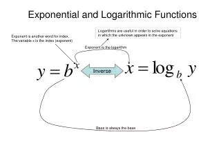
22. Logarithms • We’ve discussed exponential equations of the form y = bx (b > 0, b≠ 1) • But what about solving the same equation fory? • You may recall that y is called the logarithm of x to the base b, and is denoted logbx. • Logarithm of x to the base b y = logbxif and only ifx = by(x > 0)

23. Examples • Solve log3x= 4 for x: Solution • By definition, log3x= 4 implies x = 34 = 81. Example 2, page 338

24. Examples • Solve log164= x for x: Solution • log164= x is equivalent to 4 = 16x = (42)x= 42x, or 41 = 42x, from which we deduce that Example 2, page 338

25. Examples • Solve logx8= 3 for x: Solution • By definition, we see that logx8= 3 is equivalent to Example 2, page 338

26. Logarithmic Notation log x = log10xCommon logarithm ln x = logexNatural logarithm

27. Laws of Logarithms • If m and n are positive numbers, then

28. Examples • Given that log 2 ≈ 0.3010, log 3 ≈ 0.4771, and log 5 ≈ 0.6990, use the laws of logarithms to find Example 4, page 339

29. Examples • Given that log 2 ≈ 0.3010, log 3 ≈ 0.4771, and log 5 ≈ 0.6990, use the laws of logarithms to find Example 4, page 339

30. Examples • Given that log 2 ≈ 0.3010, log 3 ≈ 0.4771, and log 5 ≈ 0.6990, use the laws of logarithms to find Example 4, page 339

31. Examples • Given that log 2 ≈ 0.3010, log 3 ≈ 0.4771, and log 5 ≈ 0.6990, use the laws of logarithms to find Example 4, page 339

32. Examples • Expand and simplify the expression: Example 5, page 340

33. Examples • Expand and simplify the expression: Example 5, page 340

34. Examples • Expand and simplify the expression: Example 5, page 340

35. Logarithmic Function • The function defined by is called the logarithmic function with baseb. • The domain of f is the set of all positive numbers.

36. Properties of Logarithmic Functions • The logarithmic function y = logbx (b > 0, b≠ 1) has the following properties: • Its domain is (0, ). • Its range is (–, ). • Its graph passes through the point (1, 0). • It is continuous on (0, ). • It is increasing on (0, ) if b > 1 and decreasing on (0, ) if b < 1.

37. Example • Sketch the graph of the function y = ln x. Solution • We first sketch the graph of y = ex. • The required graph is the mirror image of the graph of y = ex with respect to the line y = x: y y = x y = ex y = ln x 1 x 1 Example 6, page 341

38. Properties Relating Exponential and Logarithmic Functions • Properties relating ex and ln x: eln x = x (x > 0) ln ex = x(for any real number x)

39. Examples • Solve the equation 2ex + 2 = 5. Solution • Divide both sides of the equation by 2 to obtain: • Take the natural logarithm of each side of the equation and solve: Example 7, page 342

40. Examples • Solve the equation 5 ln x + 3 = 0. Solution • Add –3 to both sides of the equation and then divide both sides of the equation by 5 to obtain: and so: Example 8, page 343

41. 5.3 Compound Interest

42. Compound Interest • Compound interest is a natural application of the exponential function to business. • Recall that simple interest is interest that is computed only on the original principal. • Thus, if I denotes the interest on a principalP (in dollars) at an interest rate of r per year for t years, then we have I = Prt • The accumulated amount A, the sum of the principal and interest after t years, is given by

43. Compound Interest • Frequently, interest earned is periodically added to the principal and thereafter earns interest itself at the same rate. This is called compound interest. • Suppose $1000 (the principal) is deposited in a bank for a term of 3 years, earning interest at the rate of 8% per year compounded annually. • Using the simple interest formula we see that the accumulated amount after the first year is or $1080.

44. Compound Interest • To find the accumulated amount A2at the end of the second year, we use the simple interest formulaagain, this time with P =A1, obtaining: or approximately $1166.40.

45. Compound Interest • We can use the simple interest formulayet again to find the accumulated amount A3 at the end of the third year: or approximately $1259.71.

46. Compound Interest • Note that the accumulated amounts at the end of each year have the following form: • These observations suggest the following general rule: • If P dollars are invested over a term of tyears earning interest at the rate of r per year compounded annually, then the accumulated amount is or:

47. Compounding More Than Once a Year • The formula was derived under the assumption that interest was compoundedannually. • In practice, however, interest is usually compoundedmore than once a year. • The interval of time between successive interest calculations is called the conversion period.

48. Compounding More Than Once a Year • If interest at a nominal a rate of r per year is compoundedm times a year on a principal of P dollars, then the simple interest rate per conversion period is • For example, the nominal interest rate is 8% per year, and interest is compounded quarterly, then or 2% per period.

49. Compounding More Than Once a Year • To find a general formula for the accumulated amount, we apply repeatedly with the interest rate i = r/m. • We see that the accumulated amount at the end of each period is as follows:

50. Compound Interest Formula • There are n = mt periods in t years, so the accumulated amount at the end oftyear is given by where A= Accumulated amount at the end of t years P= Principal r= Nominal interest rate per year m= Number of conversion periods per year t= Term (number of years)