Download
1 / 53
560 likes | 986 Vues
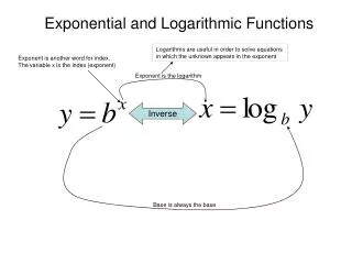
3. Exponential Functions Logarithmic Functions Exponential Functions as Mathematical Models. Exponential and Logarithmic Functions. 3.1. Exponential Functions. Exponential Function. The function defined by is called an exponential function with base b and exponent x .

E N D
3 • Exponential Functions • Logarithmic Functions • Exponential Functions as Mathematical Models Exponential and Logarithmic Functions
3.1 Exponential Functions
Exponential Function • The function defined by is called an exponential function with baseb and exponentx. • The domain of f is the set of all real numbers.
Example • The exponential function with base2 is the function with domain(–, ). • The values of f(x) for selected values of x follow:
Example • The exponential function with base2 is the function with domain(–, ). • The values of f(x) for selected values of x follow:
Laws of Exponents • Let a and b be positive numbers and let x and y be real numbers. Then,
Examples • Let f(x) = 22x – 1. Find the value of x for which f(x) = 16. Solution • We want to solve the equation 22x – 1= 16 = 24 • But this equation holds if and only if 2x – 1 = 4 giving x = .
Examples • Sketch the graph of the exponential function f(x) = 2x. Solution • First, recall that the domain of this function is the set of real numbers. • Next, putting x = 0 gives y = 20 = 1, which is the y-intercept. (There is no x-intercept, since there is no value of x for which y = 0)
Examples • Sketch the graph of the exponential function f(x) = 2x. Solution • Now, consider a few values for x: • Note that 2xapproaches zero as xdecreases without bound: • There is a horizontal asymptote at y = 0. • Furthermore, 2xincreases without bound when xincreases without bound. • Thus, the range of f is the interval(0, ).
Examples • Sketch the graph of the exponential function f(x) = 2x. Solution • Finally, sketch the graph: y 4 2 f(x) = 2x x –2 2
Examples • Sketch the graph of the exponential function f(x) = (1/2)x. Solution • First, recall again that the domain of this function is the set of real numbers. • Next, putting x = 0 gives y = (1/2)0 = 1, which is the y-intercept. (There is no x-intercept, since there is no value of x for which y = 0)
Examples • Sketch the graph of the exponential function f(x) = (1/2)x. Solution • Now, consider a few values for x: • Note that (1/2)xincreases without bound when xdecreases without bound. • Furthermore, (1/2)xapproaches zero as xincreases without bound: there is a horizontal asymptote at y = 0. • As before, the range of f is the interval(0, ).
Examples • Sketch the graph of the exponential function f(x) = (1/2)x. Solution • Finally, sketch the graph: y 4 2 f(x) = (1/2)x x –2 2
Examples • Sketch the graph of the exponential function f(x) = (1/2)x. Solution • Note the symmetry between the two functions: y 4 2 f(x) = 2x f(x) = (1/2)x x –2 2
Properties of Exponential Functions • The exponential functiony = bx (b > 0, b≠ 1) has the following properties: • Its domain is (–, ). • Its range is (0, ). • Its graph passes through the point (0, 1) • It is continuous on (–, ). • It is increasing on (–, ) if b > 1 and decreasing on (–, ) if b < 1.
The Base e • Exponential functions to the basee, where e is an irrational number whose value is 2.7182818…, play an important role in both theoretical and applied problems. • It can be shown that
Examples • Sketch the graph of the exponential function f(x) = ex. Solution • Since ex> 0 it follows that the graph ofy = exis similar to the graph ofy = 2x. • Consider a few values for x:
Examples • Sketch the graph of the exponential function f(x) = ex. Solution • Sketching the graph: y f(x) = ex 5 3 1 x –3 –1 1 3
Examples • Sketch the graph of the exponential function f(x) = e–x. Solution • Since e–x> 0 it follows that 0 < 1/e < 1 and so f(x) = e–x= 1/ex= (1/e)x is an exponential function with base less than1. • Therefore, it has a graph similar to that of y = (1/2)x. • Consider a few values for x:
Examples • Sketch the graph of the exponential function f(x) = e–x. Solution • Sketching the graph: y 5 3 1 f(x) = e–x x –3 –1 1 3
3.2 Logarithmic Functions
Logarithms • We’ve discussed exponential equations of the form y = bx (b > 0, b≠ 1) • But what about solving the same equation fory? • You may recall that y is called the logarithm of x to the base b, and is denoted logbx. • Logarithm of x to the base b y = logbxif and only ifx = by(x > 0)
Examples • Solve log3x= 4 for x: Solution • By definition, log3x= 4 implies x = 34 = 81.
Examples • Solve log164= x for x: Solution • log164= x is equivalent to 4 = 16x = (42)x= 42x, or 41 = 42x, from which we deduce that
Examples • Solve logx8= 3 for x: Solution • By definition, we see that logx8= 3 is equivalent to
Logarithmic Notation log x = log10xCommon logarithm ln x = logexNatural logarithm
Laws of Logarithms • If m and n are positive numbers, then
Examples • Given that log 2 ≈ 0.3010, log 3 ≈ 0.4771, and log 5 ≈ 0.6990, use the laws of logarithms to find
Examples • Given that log 2 ≈ 0.3010, log 3 ≈ 0.4771, and log 5 ≈ 0.6990, use the laws of logarithms to find
Examples • Given that log 2 ≈ 0.3010, log 3 ≈ 0.4771, and log 5 ≈ 0.6990, use the laws of logarithms to find
Examples • Given that log 2 ≈ 0.3010, log 3 ≈ 0.4771, and log 5 ≈ 0.6990, use the laws of logarithms to find
Examples • Expand and simplify the expression:
Examples • Expand and simplify the expression:
Examples • Expand and simplify the expression:
Examples • Use the properties of logarithms to solve the equation forx: Law 2 Definition of logarithms
Examples • Use the properties of logarithms to solve the equation forx: Laws 1 and 2 Definition of logarithms
Logarithmic Function • The function defined by is called the logarithmic function with baseb. • The domain of f is the set of all positive numbers.
Properties of Logarithmic Functions • The logarithmic function y = logbx (b > 0, b≠ 1) has the following properties: • Its domain is (0, ). • Its range is (–, ). • Its graph passes through the point (1, 0). • It is continuous on (0, ). • It is increasing on (0, ) if b > 1 and decreasing on (0, ) if b < 1.
Example • Sketch the graph of the function y = ln x. Solution • We first sketch the graph of y = ex. • The required graph is the mirror image of the graph of y = ex with respect to the line y = x: y y = x y = ex y = ln x 1 x 1
Properties Relating Exponential and Logarithmic Functions • Properties relating ex and ln x: eln x = x (x > 0) ln ex = x(for any real number x)
Examples • Solve the equation 2ex + 2 = 5. Solution • Divide both sides of the equation by 2 to obtain: • Take the natural logarithm of each side of the equation and solve:
Examples • Solve the equation 5 ln x + 3 = 0. Solution • Add –3 to both sides of the equation and then divide both sides of the equation by 5 to obtain: and so:
3.3 Exponential Functions as Mathematical Models Growth of bacteria Radioactive decay Assembly time
Applied Example: Growth of Bacteria • In a laboratory, the number of bacteria in a culture grows according to where Q0 denotes the number of bacteria initially present in the culture, k is a constant determined by the strain of bacteria under consideration, and t is the elapsed time measured in hours. • Suppose 10,000 bacteria are present initially in the culture and 60,000 present two hours later. • How many bacteria will there be in the culture at the end of four hours?
Applied Example: Growth of Bacteria Solution • We are given that Q(0) = Q0 = 10,000, so Q(t) = 10,000ekt. • At t = 2 there are 60,000 bacteria, so Q(2) = 60,000, thus: • Taking the natural logarithm on both sides we get: • So, the number of bacteria present at any time t is given by:
Applied Example: Growth of Bacteria Solution • At the end of four hours (t = 4), there will be or 360,029bacteria.
Applied Example: Radioactive Decay • Radioactive substances decay exponentially. • For example, the amount of radium present at any time t obeys the law where Q0is the initial amount present and k is a suitable positive constant. • The half-life of a radioactive substance is the time required for a given amount to be reduced by one-half. • The half-life of radium is approximately 1600 years. • Suppose initially there are 200 milligrams of pure radium. • Find the amount left after t years. • What is the amount after 800 years?
Applied Example: Radioactive Decay Solution • Find the amount left after t years. The initial amount is 200 milligrams, so Q(0) = Q0 = 200, so Q(t) = 200e–kt The half-life of radium is 1600 years, so Q(1600) = 100, thus
Applied Example: Radioactive Decay Solution • Find the amount left after t years. Taking the natural logarithm on both sides yields: Therefore, the amount of radium left after t years is:
Applied Example: Radioactive Decay Solution • What is the amount after 800 years? In particular, the amount of radium left after800 years is: or approximately 141 milligrams.