Introduction to Linear Programming in Deterministic Operations Research
Learn about LP modeling, examples, graphical interpretation, solving with Simplex in Excel, theoretical concepts, and practical applications like the Product Mix and Blending Problems. Explore historical significance and classic LP models.

Introduction to Linear Programming in Deterministic Operations Research
E N D
Presentation Transcript
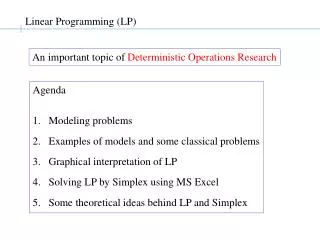
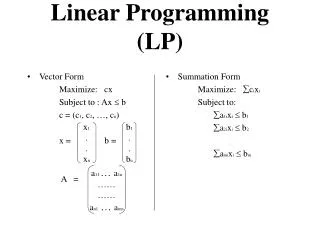
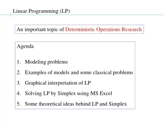
Linear Programming (LP) An important topic of Deterministic Operations Research • Agenda • Modeling problems • Examples of models and some classical problems • Graphical interpretation of LP • Solving LP by Simplex using MS Excel • Some theoretical ideas behind LP and Simplex
Example 1: Product Mix Problem Fertilizer manufacturing company, 2 types of fertilizer Type A: high phosphorus Type B: low phosphorus
Product Mix Problem: Modeling Step 1. The decision variables Daily production of Type A: x tons Type B: y tons Step 2. The objective function (maximize profit) z =15x + 10y
Product Mix Problem: Modeling.. Step 3. The constraints Limited supply of raw materials per day: Urea: 2x + y ≤ 1500 Potash: x + y ≤ 1200 Rock Phosphate: x ≤ 500
Product Mix Problem: Complete model Maximize z( x, y) = 15 x + 10y subject to 2x + y ≤ 1500 x + y ≤ 1200 x ≤ 500 x ≥ 0, y ≥ 0 Interesting Aspects: Linearity, Inequalities Feasible solutions: (0, 0), (1, 1), … Infeasible solutions: (600, 500), …
Background: Petroleum Refinery Example 2. Blending Problem Three types of petrol (minimum Octane rating: 85, 90, 95) Four types of oils (Octane rating: 68, 86, 91, 99) Blending oils petrol, with proportional Octane rating Objective: best product mix [how much of each petrol, oil to sell]
68x11 + 86x21 + 91x31 + 99x41 Its Octane Rating: ≥ 95, x11 + x21 + x31 + x41 Blending Problem: Modeling Step 1. The decision variables xij = barrels/day of oil i ( i = 1, 2, 3, or 4) to make petrol j (j = 1, 2, or 3) Total premium petrol per day = x11 + x21 + x31 + x41 68x11 + 86x21 + 91x31 + 99x41 - 95(x11 + x21 + x31 + x41) ≥ 0.
premium 45.15(x11 + x21 + x31 + x41) + 42.95(x12 + x22 + x32 + x42) + 40.99(x13 + x23 + x33 + x43) + 36.85 (4000 – (x11 + x12 + x13)) + 36.85 (5050 – (x21 + x22 + x23)) + 38.95 (7100 –(x31 + x32 + x33)) + 38.95 (4300 – (x41 + x42 + x43)) super regular Oil 1 Oil 2 Oil 3 Oil 4 Blending Problem: Modeling.. Step 2.The objective function Maximize profit Maximize revenue
Blending Problem: Modeling... Step 3.The constraints (a) The OcR constraints: 68x11 + 86x21 + 91x31 + 99x41 - 95(x11 + x21 + x31 + x41) ≥ 0 68x12 + 86x22 + 91x32 + 99x42 - 90(x12 + x22 + x32 + x42) ≥ 0 68x13 + 86x23 + 91x33 + 99x43 - 85(x13 + x23 + x33 + x43) ≥ 0
Blending Problem: Modeling.... Step 3.The constraints.. (b) Can’t use more oil than we have: x11 + x12 + x13 ≤ 4000 x21 + x22 + x23 ≤ 5050 x31 + x32 + x33 ≤ 7100 x41 + x42 + x43 ≤ 4300
Blending Problem: Modeling….. Step 3.The constraints... (c) The demand constraints: x11 + x21 + x31 + x41 ≤ 10,000 x13 + x23 + x33 + x43 ≥ 15,000 (d) Allowed values of variables xij ≥ 0 for i = 1, 2, 3, 4, and j = 1, 2, 3.
Blending Problem: complete model Maximize: 45.15(x11 + x21 + x31 + x41) + 42.95(x12 + x22 + x32 + x42) + 40.99(x13 + x23 + x33 + x43) + 36.85(4000 – (x11 + x12 + x13)) + 36.85 (5050 – (x21 + x22 + x23)) + 38.95 (7100 –(x31 + x32 + x33)) + 38.95 (4300 – (x41 + x42 + x43)) Subject to: 68x11 + 86x21 + 91x31 + 99x41 - 95(x11 + x21 + x31 + x41) ≥ 0 68x12 + 86x22 + 91x32 + 99x42 - 90(x12 + x22 + x32 + x42) ≥ 0 68x13 + 86x23 + 91x33 + 99x43 - 85(x13 + x23 + x33 + x43) ≥ 0 x11 + x12 + x13 ≤ 4000 x21 + x22 + x23 ≤ 5050 x31 + x32 + x33 ≤ 7100 x41 + x42 + x43 ≤ 4300 x11 + x21 + x31 + x41 ≤ 10,000 x13 + x23 + x33 + x43 ≥ 15,000 xij ≥ 0 for I = 1, 2, 3, 4, and j = 1, 2, 3. Octane rating Supply Demand
Example 3: Transportation problem Background: Company has several factories (sinks), and several suppliers (sources) Objective: Minimize the cost of transportation
Transportation problem: the model Step 1. The decision variables xij= amount of ore shipped from mine i to plant j per day. Step 2:The objective function Minimize the transportation costs: Minimize: 11x11 + 8x12 + 2x13 + 7x21 + 5x22 + 4x23
Transportation problem: the model.. Step 3.The constraints (a) Shipment from each mine less than daily production x11 + x12 + x13 ≤ 800 [capacity of mine 1] x21 + x22 + x23 ≤ 300 [capacity of mine 2] (b) Demand of each plant must be met x11 + x21 ≥ 400 [demand at plant 1] x12 + x22 ≥ 500 [demand at plant 2] x13 + x23 ≥ 200 [demand at plant 3] (c) Decision variables can’t be negative xij ≥ 0, for all i= 1, 2, j = 1, 2, 3.
Transportation problem: historical note Kantorovich in USSR in the 1930’s, Koopmans in 1940’s Dantzig in 1950’s Simplex method Kantorovich and Koopmans, Nobel prize (Economics) in 1975
Point in a 1D space: x = c c 0 y 3 2x+3y = 9 2x+3y = 3 2 2x+3y = 6 2x+3y = 0 1 x 3 4.5 (0,0) 1.5 The Geometry of Linear Programs Line in 2D: ax + by = c
z 1 Plane x + y + z = 1 Plane: x + y + z = 2 z Plane: x + y + z = 0 1 x 1 1 1 y y 1 x The Geometry of Linear Programs Plane in 3D: ax + by + cz = d
y 3 2x+3y > 6 2 2x+3y < 6 1 x 4.5 3 1.5 (0,0) 2x+3y = 6 The Geometry of Linear Programs Hyper-plane in n-Dimensions: a1x1 + a2x2 + … + anxn = c ?? 2-D Half spaces:
y y ≥0 1500 1000 500 x ≥0 x 500 Feasible set 1000 (0,0) 1500 x + y ≤ 1200 x ≤ 500 2x+y ≤ 1500 The Geometry of LP: Product Mix revisited max z( x, y) = 15 x + 10y ST 2x + y ≤ 1500 x + y ≤ 1200 x ≤ 500 x ≥ 0, y ≥ 0
y y ≥0 15x + 10y = 5000 1500 15x + 10y = 13,500 1000 15x + 10y = 0 (300, 900) 500 x ≥0 x 500 Feasible set 1000 (0,0) 1500 x + y ≤ 1200 x ≤ 500 2x+y ≤ 1500 The Geometry of LP: Product Mix revisited max z( x, y) = 15 x + 10y ST 2x + y ≤ 1500 x + y ≤ 1200 x ≤ 500 x ≥ 0, y ≥ 0 Try point: x = 0, y = 0:
Summary 1. LP formulations are very common in modern industry 2. Beautiful connection between Algebra and Geometry 3. Geometry not useful for > 3 variables 4. Practical problems: 1000’s of variables (see next slide) 5. Need Algebraic method !
Some real world examples of LP Military patient evacuation problem The US Air Force Military Airlift Command (MAC) has a patient evacuation problem that can be modeled as an LP. They use this model to determine the flow of patients moved by air from an area of conflict to army bases and hospitals. The objective is to minimize the time that patients are in the air transport system. The constraints are: - all patients that need transporting must be transported - limits on the size and composition of hospitals, capacity of air fleet, air-lift points MAC have generated a series of problems based on the number of time periods (days). A 50 day problem consists of an LP with 79,000 constraints and 267,000 variables. This LP can be solved (using a fast computer) in approximately 10 Hours
Some real world examples of LP.. Military logistics planning The US Department of Defense Joint Chiefs of Staff have a logistics planning problem that models the feasibility of supporting military operations during a crisis. The problem is to determine if different materials (called movement requirements) can be transported overseas within strict time windows. The LP includes capacities at embarkation and debarkation ports, capacities of the various aircraft and ships that carry the movement requirements and penalties for missing delivery dates. A typical problem of this type may consider 15 time periods, 12 ports of embarkation, 7 ports of debarkation and 9 different types of vehicle for 20,000 movement requirements. This resulted in an LP with 20,500 constraints and 520,000 variables. This LP can be solved in approximately 75 minutes
Some real world examples of LP... Airline crew scheduling (American Airlines) Within a fixed airline schedule (the schedule changing twice a year typically) each flight in the schedule can be broken down into a series of flight legs. A flight leg comprises a takeoff from a specific airport at a specific time to the subsequent landing at another airport at a specific time. For example a flight from HK Bangkok Phuket has two legs. A key point is that these flight legs may be flown by different crews. For crew scheduling, aircraft types have been pre-assigned (not all crews can fly all types). For a given aircraft type and a given time period (the schedule repeats over a 1 week period) we must ensure that all flight legs for a particular aircraft type can have a crew assigned. Note here that by crew we mean not only the pilots/flight crew but also the cabin service staff, typically these work together as a team and are kept together over a schedule. There are restrictions on how many hours the crews (pilots and others) can work. A potential crew schedule is a series of flight legs that satisfies these restrictions. All such potential crew schedules can have a cost assigned to them. Usually a crew schedule ends up with the crew returning to their home base, e.g. A-D and D-A in crew schedule 1 above. A crew schedule such as 2 above (A-B and B-C) typically includes as part of its associated cost the cost of returning the crew (as passengers) to their base. Such carrying of crew as passengers (on their own airline or on another airline) is called deadheading. For our American Airlines problem the company has a database with 12 millionpotential crew schedules. The objective is to select the combination of schedules (out of the 12 million) which shall minimize costs. The constraints are to ensure that all flight legs have a crew assigned to them, and work restrictions are violated. One case of this problem was formulated as an LP, with 12 million variables, and 750 constraints. [Note: a small percentage improvement of the schedule ten's of millions of dollars!] This LP could be solved in approximately 27 minutes using a software called OSL next: How to solve LP’s using MS Excel