LINEAR PROGRAMMING (LP)

1. LINEAR PROGRAMMING (LP) Lecture 10 Dr. Arshad Zaheer

2. TWO-VARIABLE LP MODEL EXAMPLE: “ THE GALAXY INDUSTRY PRODUCTION” • Galaxy manufactures two toy models: • Space Ray. • Zapper. • Resources are limited to • 1200 pounds of special plastic. • 40 hours of production time per week.

3. Marketing requirement • Total production cannot exceed 800 dozens. • Number of dozens of Space Rays cannot exceed number of dozens of Zappers by more than 450. • Technological input • Space Rays requires 2 pounds of plastic and 3 minutes of labor per dozen. • Zappers requires 1 pound of plastic and 4 minutes of labor per dozen.

4. Current production plan calls for: • Producing as much as possible of the more profitable product, Space Ray ($8 profit per dozen). • Use resources left over to produce Zappers ($5 profit per dozen). • The current production plan consists of: Space Rays = 550 dozens Zapper = 100 dozens Profit = 4900 dollars per week

5. A Linear Programming Model can provide an intelligent solution to this problem

6. SOLUTION • Decisions variables: • X1 = Production level of Space Rays (in dozens per week). • X2 = Production level of Zappers (in dozens per week). • Objective Function: • Weekly profit, to be maximized

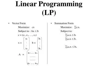
7. The Linear Programming Model Max 8X1 + 5X2 (Weekly profit) subject to 2X1 + 1X2 < = 1200 (Plastic) 3X1 + 4X2 < = 2400 (Production Time) X1 + X2 < = 800 (Total production) X1 - X2 < = 450 (Mix) Xj> = 0, j = 1,2 (Nonnegativity)

8. Feasible Solutions for Linear Programs • The set of all points that satisfy all the constraints of the model is called FEASIBLE REGION

9. Using a graphical presentation we can represent all the constraints, the objective function, and the three types of feasible points.

10. The plastic constraint: 2X1+X2<=1200 The Plastic constraint Productionmix constraint: X1-X2<=450 X2 1200 Total production constraint: X1+X2<=800 Infeasible 600 Feasible Production Time 3X1+4X2<=2400 X1 600 800

11. Solving Graphically for an Optimal Solution

12. Profit = $ 000 Recall the feasible Region We now demonstrate the search for an optimal solution Start at some arbitrary profit, say profit = $2,000... Then increase the profit, if possible... X2 1200 ...and continue until it becomes infeasible Profit =$5040 4, 2, 3, 800 600 X1 400 600 800

13. X2 1200 Let’s take a closer look at the optimal point 800 Infeasible 600 Feasible region Feasible region X1 400 600 800

14. The plastic constraint: 2X1+X2<=1200 The Plastic constraint Productionmix constraint: X1-X2<=450 X2 1200 Total production constraint: X1+X2<=800 Infeasible 600 A (0,600) B (480,240) Feasible Production Time 3X1+4X2<=2400 C (550,100) E O (0,0) D (450,0) X1 600 800

15. To determine the value for X1 and X2 at the optimal point, the two equations of the binding constraint must be solved.

16. Productionmix constraint: X1-X2<=450 The plastic constraint: 2X1+X2<=1200 2X1+X2=1200 3X1+4X2=2400 X1= 480 X2= 240 Production Time 3X1+4X2<=2400 2X1+X2=1200 X1-X2=450 X1= 550 X2= 100

17. By Compensation on : Max 8X1 + 5X2 The maximum profit (5040) will be by producing: Space Rays = 480 dozens, Zappers = 240 dozens

18. Illustration

19. Illustration

20. A manager must decide on the mix of products to produce for the coming week. Product A requires three minutes per unit for molding, two minutes per unit for painting, and one minute for packing. Product B requires two minutes per unit for molding, four minutes for painting, and three minutes per unit for packing. There will be 600 minutes available for molding, 600 minutes for painting, and 420 minutes for packing. Both products have contributions of $1.50 per unit.

21. Requirements: • Algebraically state the objective and constraints of this problem. • Plot the constraints on the grid and identify the feasible region. • Maximize objective function

22. Let X1 = Product A X2 = Product B

23. Graphical Method 1.Algebraically state the objective and constraints of this problem. Maximize Z = 1.50X1+1.50X2 Subject to 3X1 + 2X2 < 600 (Molding constraint)……(I) 2X1 + 4X2 < 600(Painting constraint)……(II) X1 + 3X2 < 420(Packing constraint)……(III) X1, X2 > 0 (Non-negative constraint)

24. Graphical Method (cont.) • Plot the constraints on the coordinate Axis and identify the feasible region. Solution • Find the coordinates (X1, X2) for each constraint as well as for objective function and draw them on the same coordinate axis.

25. Graphical Method (cont.)

26. Graphical Method (cont.) Objective Function

27. Graphical Method (cont.) X2 The Optimal Solution can be found on corners 3X1 + 2X2 < 600 (Molding constraint)) 300 250 X1 + 3X2 < 420 (Packing constraint) 200 150 A Objective Function 100 B Optimal Point Feasible Region C 50 O D 2X1 + 4X2 < 600 (Painting constraint) X1 100 200 300 400 500

28. Graphical Method (cont.) • One of the corner point (B) is the intersection of following two lines 2X1 + 4X2 < 600 (1) X1 + 3X2 < 420 (2) We can find their solution by following methods; • Substitution • Addition • Subtraction Here we use the subtraction method step 1: multiply equation 2 with 2 and rewrite

29. Graphical Method (cont.) 2X1 + 4X2 = 600 (1) -2X1 + 6X2 = - 840 (2) -2X2= - 240 X2= 120 By putting X2= 120 in equation 1 we will get 2(X1) + 4(120) = 600 X1= 60 B (60, 120)

30. Graphical Method (cont.) • Other of the corner point (C) is the intersection of following two lines 3X1 + 2X2 < 600 (I) 2X1 + 4X2 < 600 (II) step 1: multiply equation I with 2, rewrite and subtract

31. Graphical Method (cont.) 6X1 + 4X2 = 1200 + 2X1 + 4X2 = + 600 4X1= 600 X1= 150 By putting X1= 150 in equation 1 we will get 3(150) + 2X2 = 600 X2= 75 C (150, 75)

32. The maximum profit (5040) will be by producing: Space Rays = 480 dozens, Zappers = 240 dozens

33. Formulation of Linear Programming • A company wants to purchase at most 1800 units of a product. There are two types of the product M1 and M2 available. M1 occupies 2ft3, costs Rs. 4 and the company makes the profit of Rs. 3. M2 occupies 3ft3, costs Rs. 5, and the company makes the profit of Rs. 4. If the budget is Rs. 5500/= and warehouse has 3000 ft3for the products. Requirement Formulate the problem as linear programming problem.

34. Solution Let X1 = Product M1 X2 = Product M2

35. Formulation of Linear Programming (Cont.) Step 1 • Key decision to be made • Maximization of Profit • Identify the decision variables of the problem Let X1 = Product M1 X2 = Product M2

36. Formulation of Linear Programming (Cont.) Step 2 • Formulate the objective function to be optimized • For maximization the objective function is based on profit • Profit from M1 = 3X1 • Profit from M2 = 4X2 so our objective function will be like this Maximize Z = 3X1+4X2

37. Formulation of Linear Programming (Cont.) Step 3 • Formulate the constraints of the problem • For area the maximum availability is 3000 ft3, and area required for M1 (X1) is 2 ft3 where for product M2 (X2) is 3 ft3. so the constraint become as under • 2X1 + 3X2< 3000 • For cost the maximum availability is Rs. 5500, Product M (X1) required Rs. 4 per unit and product M2 (X2) required Rs. 5 per unit so the constraint become as under • 4X1 +5 X2<5500

38. Formulation of Linear Programming (Cont.) • Third condition: Company wants to purchase at most 1800 units of a product This is the production constraints that the company must produce at most 1800 of the product and the product is composed of X1 and X2, so the mixture of these two X1 + X2 ≤ 1800

39. Formulation of Linear Programming (Cont.) Step 4 - Add non-negativity restrictions or constraints The decision variables should be non negative, which can be expressed in mathematical form as under; X1, x2 > 0

40. Formulation of Linear Programming (Cont.) • The whole Linear Programming model is as under; Maximize Z = 3X1+4X2 (Objective Function) Subject to 2X1 + 3X2 < 3000 (Area Constraint) 4X1 + 5 X2 < 5500 (Cost Constraint) X1 + X2 ≤ 1800 (Product Constraint) X1,X2 > 0 (Non-Negative Constraint)

41. Thank You