Linear Programming
Linear Programming. Dragan Jovicic Harvinder Singh. Introduction to LP. Linear programming (LP) problems are optimization problems where the objective function and the constraints of the problem are all linear.

Linear Programming
E N D
Presentation Transcript
Linear Programming Dragan Jovicic Harvinder Singh
Introduction to LP • Linear programming (LP) problems are optimization problems where the objective functionand the constraintsof the problem are all linear. • Many practical problems in operations research can be expressed as linear programming problems. • A lot of work is generated on the research of specialized algorithms for the solutions of specific LP problems. • In mathematical optimization theory, the simplex algorithm of George Dantzig is the fundamental technique for numerical solution of the LP problem.
Outline • Introduction • Standard Form • Matrix Form • Example of LP formulation • Example 1 • Augmented form (slack form) • Example 2 • Theory • Simplex algorithm
Guidelines for Model Formulation • Understand the problem thoroughly. • Describe the objective. • Describe each constraint. • Define the decision variables. • Write the objective in terms of the decision variables. • Write the constraints in terms of the decision variables.
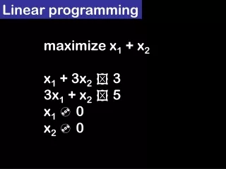
Standard form • Standard form is a basic way of describing a LP problem. • It consists of 3 parts: • A linear function to be maximized maximize c1x1 + c2x2 + … + cnxn • Problem constraints subject to a11x1 + a12x2 + … + a1nxn< b1 a21x1 + a22x2 + … + a2nxn< b2 … am1x1 + am2x2 + … + amnxn < bm • Non-negative variables e.g. x1, x2 > 0
Matrix form • The problems is usually expressed in matrix form and then it becomes: maximize cTx subject to Ax < b, x >0 Other forms, such as minimization problems, problems with constraints on alternative forms, as well as problems involving negative variables can always be rewritten into an equivalent problem in standard form.
Example of LP formulation : A Maximization Problem LP Formulation Maximize 5x1 + 7x2 s.t. x1< 6 2x1 + 3x2< 19 x1 + x2< 8 x1, x2> 0 Standard Form Max 5x1 + 7x2 + 0s1 + 0s2 + 0s3 s.t. x1 + s1 = 6 2x1 + 3x2+ s2 = 19 x1 + x2 + s3 = 8 x1, x2 , s1 , s2 , s3> 0
Example 1 • Suppose that a farmer has a piece of farm land, say A square kilometers large, to be planted with either wheat or barley or some combination of the two. The farmer has a limited permissible amount F of fertilizer and P of insecticide which can be used, each of which is required in different amounts per unit area for wheat (F1, P1) and barley (F2, P2). Let S1 be the selling price of wheat, and S2 the price of barley. If we denote the area planted with wheat and barley with x1 and x2 respectively, then the optimal number of square kilometers to plant with wheat vs. barley can be expressed as a linear programming problem: ->
Example 1 cont. maximize S1x1 + S2x2( maximize the revenue – this is the “objective function”) subject to x1 +x2< A (limit on total area) F1x1 + F2x2< F (limit on fertilizer) P1x2 + P2x2< P (limit on insecticide) x1 >= 0, x2> 0 (cannot plant a negative area) which in matrix form becomes maximize subject to
Augmented form (slack form) • Linear programming problems must be converted into augmented form before being solved by the simplex algorithm. This form introduces non-negative slack variables to replace non-equalities with equalities in the constraints. The problem can then be written on the following form: Maximize Z in:
Example 1 (slack form) The example 1 above becomes as follows when converted Into augmented form: maximize S1x1 + S2x2(objective function) subject tox1 +x2+ x3 = A (augmented constraint) F1x1 + F2x2< F + x4 = F (augmented constraint) P1x2 + P2x2 + x5= P (augmented constraint) where x3,x4,x5 are (non-negative) slack variables. Which in matrix form becomes: Maximize Z in:
THEORY * Geometrically, the linear constraints define a convex polyhedron, which is called the feasible region. The linear objective function implies that an optimal solution can only occur at a boundary point of the feasible region. * There are two situations in which no optimal solution can be found: 1. if the constraints contradict each other (for instance, x ≥ 2 and x ≤ 1) then the feasible region is empty and there can be no optimal solution, since there are no solutions at all. In this case, the LP is said to be infeasible. 2. Alternatively, the polyhedron can be unbounded in the direction of the objective function (for example: maximize x1 + 3 x2 subject to x1 ≥ 0, x2 ≥ 0, x1 + x2 ≥ 10), in which case there is no optimal solution since solutions with arbitrarily high values of the objective function can be constructed.
THEORY cont. * The optimum is always attained at a vertex of the polyhedron. However, the optimum is not necessarily unique: it is possible to have a set of optimal solutions covering an edge or face of the polyhedron, or even the entire polyhedron (This last situation would occur if the objective function were constant).
Simplex algorithm • In mathematical optimization theory, the simplex algorithm of George Dantzig is the fundamental technique for numerical solution of the linear programming problem. • The simplex algorithm solves LP problems by constructing an admissible solution at a vertex of the polyhedron, and then walking along edges of the polyhedron to vertices with successively higher values of the objective function until the optimum is reached. • The elementary simplex method is the name of Dantzig's original (1947) algorithm, with the following rules applied to the standard form: Min {cx: Ax=b, x >= 0}. Let dj = reduced cost of xj; terminate if dj> 0 for all j. Select dj < 0 as one of greatest magnitude. In the associated column (j) of the tableau, compute the min ratio: xi / a(i, j): a(i, j) > 0. (If a(., j) <= 0, LP is unbounded). Enter xj into the basic set, in exchange for xi, and update the tableau. Version of simplex algorithm and the source code can be found at http://www-fp.mcs.anl.gov/otc/Guide/CaseStudies/simplex/applet/SimplexTool.html

