Communication Models for Parallel Computer Architectures
Explore the two distinct models for CPU communication in parallel computer systems - multiprocessors and multicomputers. Learn about shared memory, interconnection networks, and switching strategies.

Communication Models for Parallel Computer Architectures
E N D
Presentation Transcript
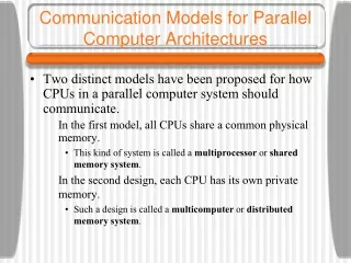
Communication Models for Parallel Computer Architectures • Two distinct models have been proposed for how CPUs in a parallel computer system should communicate. • In the first model, all CPUs share a common physical memory. • This kind of system is called a multiprocessor or shared memory system. • In the second design, each CPU has its own private memory. • Such a design is called a multicomputer or distributed memory system.
Multiprocessors • Consider a program to find all of the objects in a bit-map image. • One copy of the image is kept in memory. • Each CPU runs a single process which inspects one section of the image. • Some objects occupy multiple sections, so it is essential that each process have access to the entire image. • Example multiprocessors include: • Sun Enterprise 1000 • Sequent NUMA-Q • SGI Origin 2000 • HP/Convex Exemplar
Multicomputers • In a multicomputer solving the same problem, each CPU has a section of the image in its local memory. • If the CPUs need to follow an object across the border, they must request the information from a neighboring CPU. • This is done via message passing. • Programming multicomputers is more difficult than programming multiprocessors, but they are more scalable. • Building a multicomputer with 10,000 CPUs is straightforward.
Multicomputers • Example multicomputers include: • IBM SP/2 • Intel/Sandia Option Red • Wisconsin COW • Much research focuses on hybrid systems combining the best of both worlds. • Shared memory might be implemented at a higher-level than the hardware. • The operating system might simulate a shared memory by providing a single system-wide paged shared address space. • This approach is called DSM (Distributed Shared Memory).
Shared Memory • Each machine has its own virtual memory and its own page table. • When a CPU does a LOAD or STORE on a page it does not have, a trap to the OS occurs. • The OS locates the page and asks the CPU currently holding it to unmap the page and send it over the interconnection network. • When it arrives, the page is mapped in and the faulting instruction restarted. • A third possibility is to have a user-level runtime system implement a form of shared memory.
Shared Memory • The programming language provides a shared memory abstraction implemented by the compiler and runtime system. • The Linda model is based on the abstraction of a shared space of tuples. • Processes can input a tuple from the shared tuple space or output a tuple to the shared tuple space. • The Orca model allows shared generic objects. • Processes can execute object-specific methods on shared objects. • When a change occurs to the internal state of some object, it is up to the runtime system to simultaneously update all copies of the object.
Interconnection Networks • Multicomputers are held together by interconnection networks which move packets between CPUs and memory. • The CPUs and memory modules of multiprocessors are also interconnected. • Interconnection networks consist of: • CPUs • Memory modules • Interfaces • Links • Switches
Interconnection Networks • The links are the physical channels over which bits move. They can be • electrical or optical fiber • serial or parallel • simplex, half-duplex, or full duplex • The switches are devices with multiple input ports and multiple output ports. • When a packet arrives at an input port on a switch some bits are used to select the output port to which the packet is sent.
Switching • An interconnection network consists of switches and wires connecting them. • The following slide shows an example. • Each switch has four input ports and four output ports. • In addition each switch has some CPUs and interconnect circuitry. • The job of the switch is to accept packets arriving on any input port and send each one out on the correct output port. • Each output port is connected to an input port of another switch by a parallel or serial line.
Switching • Several switching strategies are possible. • In circuit switching, before a packet is sent, the entire path from the source to the destination is reserved in advance. • All ports and buffers are claimed, so that when transmission starts, all necessary resources are guaranteed to be available and the bits can move at full speed from the source, through the switches to the destination. • In store-and-forward packet switching, no advance reservation is needed. • The source sends a complete packet to the first switch where it is stored in its entirety. • The switches may need to buffer packets if an output port is busy.
Communication Methods • When a program is split up into pieces, the pieces (processes) often need to communicate with one another. • This communication can be done in one of two ways: • shared variables • explicit message passing • Logical sharing of variables is possible even on a multicomputer. • Message passing is easy to implement on a multiprocessor by simply copying from the sender to the receiver.
Message Passing Modes • Messaging systems can be either persistent or transient • Are messages retained when the senders and/or receivers stop executing? • Can also be either synchronous or asynchronous • Blocking vs. non-blocking
Persistent Communication • Persistent communication of letters back in the days of the Pony Express.
Persistence and Synchronicity in Communication • Persistent asynchronous communication • Persistent synchronous communication 2-22.1
Persistence and Synchronicity in Communication • Transient asynchronous communication • Receipt-based transient synchronous communication 2-22.2
Persistence and Synchronicity in Communication • Delivery-based transient synchronous communication at message delivery • Response-based transient synchronous communication
Remote Procedure Call (RPC) • Developed by Birrell and Nelson (1984). • In multiprocessor systems the client code for copying a file is quite different from the normal centralized (uniprocessor) code. • Let’s make the client server request-reply look like a normal procedure call and return. • Notice that getchar in the centralized version turns into a read system call. The following is for Unix: • read looks like a normal procedure to its caller.
Remote Procedure Call (RPC) • read is a user mode program. • read manipulates registers and then does a trap to the kernel. • After the trap, the kernel manipulates registers and then does a C-language routine and lots of work gets done (drivers, disks, etc). • After the I/O, the process get unblocked, the kernel read manipulates registers, and returns. The user mode read manipulates registers and returns to the original caller. • Let’s do something similar with request reply:
Remote Procedure Call (RPC) • User (client) does a subroutine call to getchar (or read). • Client knows nothing about messages. • We link in a user mode program called the client stub (analogous to the user mode read above). • This takes the parameters to read and converts them to a message (marshalls the arguments). • Sends a message to machine containing the server directed to a server stub. • Does a blocking receive (of the reply message).
Remote Procedure Call (RPC) • The server stub is linked with the server. • It receives the message from the client stub. • Unmarshalls the arguments and calls the server (as a subroutine). • The server procedure does what it does and returns (to the server stub). • Server knows nothing about messages • Server stub now converts this to a reply message sent to the client stub. • Marshalls the arguments.
Remote Procedure Call (RPC) • Client stub unblocks and receives the reply. • Unmarshalls the arguments. • Returns to the client. • Client believes (correctly) that the routine it calls has returned just like a normal procedure does.
Passing Value Parameters (1) • Steps involved in doing remote computation through RPC 2-8
Remote Procedure Call (RPC) • Heterogeneity: Machines have different data formats. • How can we handle these differences in RPC? • Have conversions between all possibilities. • Done during marshalling and unmarshalling. • Adopt a standard and convert to/from it.
Passing Value Parameters (2) • Original message on the Pentium • The message after receipt on the SPARC • The message after being inverted. The little numbers in boxes indicate the address of each byte
Remote Procedure Call (RPC) • Pointers: Avoid them for RPC! • Can put the object pointed to into the message itself (assuming you know its length). • Convert call-by-reference to copyin/copyout • If we have in or out parameters (instead of in out) can eliminate one of the copies • Change the server to handle pointers in a special way. • Callback to client stub
Registering and name servers • As we said before, we can use a name server. • This permits the server to move using the following process. • deregister from the name server • move • reregister • This is sometimes called dynamic binding.
Registering and name servers • The client stub calls the name server (binder) the first time to get a handle to use for the future. • There is a callback from the binder to the client stub if the server deregisters or we could have the attempt to use the handle fail so that the client stub will go to the binder again.
How does a programmer create a program with RPC? • uuidgen generates a unique identifier for the RPC • Include it in an IDL (interface description language file) and describe the interface for the RPC in the file as well • Write the client and server code • Client and server stubs are generated from the IDL file automatically • Link things together and run on desired machines
Writing a Client and a Server • The steps in writing a client and a server in DCE RPC. 2-14
Processor Allocation • Processor Allocation • Decide which processes should run on which processors. • Could also be called process allocation. • We assume that any process can run on any processor.
Processor Allocation • Often the only difference between different processors is: • CPU speed • CPU speed and amount of memory • What if the processors are not homogeneous? • Assume that we have binaries for all the different architectures. • What if not all machines are directly connected • Send process via intermediate machines
Processor Allocation • If we have only PowerPC binaries, restrict the process to PowerPC machines. • If we need machines very close for fast communication, restrict the processes to a group of close machines. • Can you move a running process or are processor allocations done at process creation time? • Migratory allocation algorithms vs. non migratory.
Processor Allocation • What is the figure of merit, i.e. what do we want to optimize in order to find the best allocation of processes to processors? • Similar to CPU scheduling in centralized operating systems. • Minimize response time is one possibility.
Processor Allocation • We are not assuming all machines are equally fast. • Consider two processes. P1 executes 100 millions instructions, P2 executes 10 million instructions. • Both processes enter system at time t=0 • Consider two machines A executes 100 MIPS, B 10 MIPS • If we run P1 on A and P2 on B each takes 1 second so average response time is 1 sec. • If we run P1 on B and P2 on A, P1 takes 10 seconds P2 .1 sec. so average response time is 5.05 sec. • If we run P2 then P1 both on A finish at times .1 and 1.1 so average response time is .6 seconds!!
Processor Allocation • Minimize response ratio. • Response ratio is the time to run on some machine divided by time to run on a standardized (benchmark) machine, assuming the benchmark machine is unloaded. • This takes into account the fact that long jobs should take longer. • Maximize CPU utilization • Throughput • Jobs per hour • Weighted jobs per hour
Processor Allocation • If weighting is CPU time, we get CPU utilization • This is the way to justify CPU utilization (user centric) • Design issues • Deterministic vs. Heuristic • Use deterministic for embedded applications, when all requirements are known a priori. • Patient monitoring in hospital • Nuclear reactor monitoring • Centralized vs. distributed • We have a tradeoff of accuracy vs. fault tolerance and bottlenecks.
Processor Allocation • Optimal vs. best effort • Optimal normally requires off line processing. • Similar requirements as for deterministic. • Usual tradeoff of system effort vs. result quality. • Transfer policy • Does a process decide to shed jobs just based on its own load or does it have (and use) knowledge of other loads? • Also called local vs. global • Usual tradeoff of system effort (gather data) vs. result quality.
Processor Allocation • Location policy • Sender vs. receiver initiated. • Sender initiated - uploading programs to a compute server • Receiver initiated - downloading Java applets • Look for help vs. look for work. • Both are done.
Processor Allocation • Implementation issues • Determining local load • Normally use a weighted mean of recent loads with more recent weighted higher.
Processor Allocation • Example algorithms • Min cut deterministic algorithm • Define a graph with processes as nodes and IPC traffic as arcs • Goal: Cut the graph (i.e some arcs) into pieces so that • All nodes in one piece can be run on one processor • Memory constraints • Processor completion times • Values on cut arcs are minimized
Processor Allocation • Minimize the max • minimize the maximum traffic for a process pair • Minimize the sum • minimize total traffic • Minimize the sum to/from a piece • don't overload a processor • Minimize the sum between pieces • minimize traffic for processor pair • Tends to get hard as you get more realistic
Processor Allocation • Up-down centralized algorithm • Centralized table that keeps "usage" data for a user, the users are defined to be the workstation owners. Call this the score for the user. • The goal is to give each user a fair share. • When user requests a remote job, if a workstation is available it is assigned. • For each process a user has running remotely, the user's score increases by a fixed amount each time interval.
Processor Allocation • When a user has an unsatisfied request pending (and none being satisfied), the score decreases (it can go negative). • If no requests are pending and none are being satisfied, the score is bumped towards zero. • When a processor becomes free, assign it to a requesting user with the lowest score.