Impedance measurements and simulations of the TCLD collimator prototype
Impedance measurements and simulations of the TCLD collimator prototype. F. Giordano, L. Teofili and N. Biancacci. Measurement techniques:. Probe measurement Wire measurement. Simulations tools:. CST HFSS. Probe Measurements.

Impedance measurements and simulations of the TCLD collimator prototype
E N D
Presentation Transcript
Impedancemeasurements and simulations of the TCLD collimatorprototype F. Giordano, L. Teofili and N. Biancacci
Measurement techniques: Probe measurement Wire measurement Simulations tools: • CST • HFSS
Probe Measurements • Probes connected to the VNA are inserted in a DUT (TCLD). • 2 different kind of probes for electric and magnetic modes. • The probes are moved in order to spot the modes of the DUT. • The probes themselves introduce resonances, these resonances shift with varying the position of the probes.
Wire Measurements Wire is installed in the DUT acting as source for the EM fields. A weight is used in order to stretch the wire A transverse impedance study can be done for each mode.
Simulations: The CST Model Section Cut Lateral RF-shielding Insertion RF-Fingers Tungsten Jaws Cooling System Jaws Motions System BPM The surrounding tank has been modeled as a vacuum brick, the geometry of the collimator has bees trimmed subsequently on the vacuum.
Simulations: The CST Model Front View Insertion Fingers Lateral RF-Fingers Due to the required jaws motion and design constraints the RF-fingers cannot be continuous in the geometry. The discontinuities can be possible leaking part.
Different Operational Configurations Beam Since the collimators have always the same structure, only the case P 7-1 and P 2-1 were simulated being the most conservative.
Simulations The presented model was simulated in the outlined configurations trough the Eigenmode solver of the software CST and HFSS. The two software have showed an amazing agreement on the results in both the configurations, particularly on the mode with a frequency below 500 MHz.
Measurements and simulation well match: for every measured mode it is possible to find a correspondence with one or more simulated modes (Except for some rare exception).
Mode Geometry The Computed Shunt Impedance is really small, the modes should not be dangerous. However, further analysis are on going to understand if they are transverse modes.
Transverse mode fitting Wire position: -0.5mm Varying the transverse position of the wire Wire position: 0.5mm Wire position: 0mm
Conclusions • There is a very good agreement between simulations and measurements • All the mode measure have been predicted by the simulations • The study of the impact of the modes on the power loss and beam stability is still on going
AOB: CST EigenMode Solver CST EigenMode 3 Modes to Compute Logfile CST EigenMode 5 Modes to Compute Logfile ---------------------------------------------------------------------- Total number of passes : 7 Mesh adaptation pass : 7 ---------------------------------------------------------------------- Solver time : 106 s Number of mesh cells : 125569 Number of d.o.f. : 871924 Relative estimated error : 0.001201 ---------------------------------------------------------------------- ---------------------------------------------------------------------- Total adaptive computation time: 0h : 6m : 8s Desired accuracy limit reached, mesh adaptation stopped. ---------------------------------------------------------------------- Eigenmode solver results: Mode Frequency Accuracy 1 0.2124568 GHz 1.238e-04 2 0.3189764 GHz 1.489e-08 3 0.3885921 GHz 1.34e-07 *** Warning *** The eigenmode solver stops due to maximal number of iterations. (Adaptation is stopped as well.) 1 0.09624635 GHz 2.482e-07 2 0.1478878 GHz 3.567e-08 3 0.1675404 GHz 6.846e-08 4 0.2126847 GHz 1.132e-07 5 0.3156739 GHz 8.086e-08 Marked 179 of 54279 for refinement. Marked 17 of 54279 for refinement. For some elements the curvature had to be reduced to maintain the quality of the mesh. More... Refinement successful Pass 4: Eigenmode solver results: Mode Frequency Accuracy 1 0.2126842 GHz 1.368e-05 2 0.3156732 GHz 1.405e-08 3 0.3887875 GHz 1.15e-07 4 0.4349508 GHz 2.069e-07 5 0.4467135 GHz 3.259e-06 Marked 4648 of 55302 for refinement. Marked 10 of 55302 for refinement. For some elements the curvature had to be reduced to maintain the quality of the mesh. More... Refinement successful Pass 5: Eigenmode solver results: Mode Frequency Accuracy 1 0.1050053 GHz 6.273e-07 2 0.2130525 GHz 1.701e-08 3 0.2443145 GHz 2.769e-08 4 0.2566526 GHz 3.611e-07 5 0.3160113 GHz 2.661e-07