Download
1 / 10
100 likes | 298 Vues
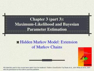
Chapter 3 (part 3): Maximum-Likelihood and Bayesian Parameter Estimation. Hidden Markov Model: Extension of Markov Chains. All materials used in this course were taken from the textbook “Pattern Classification” by Duda et al., John Wiley & Sons, 2001

E N D
Chapter 3 (part 3): Maximum-Likelihood and Bayesian Parameter Estimation Hidden Markov Model: Extension of Markov Chains All materials used in this course were taken from the textbook “Pattern Classification” by Duda et al., John Wiley & Sons, 2001 with the permission of the authors and the publisher
Hidden Markov Model (HMM) • Interaction of the visible states with the hidden states bjk= 1 for all j where bjk=P(Vk(t) | j(t)). • 3 problems are associated with this model • The evaluation problem • The decoding problem • The learning problem CSE 616 Applied Pattern Recognition, Chapter 3, Section 3.10
The evaluation problem It is the probability that the model produces a sequence VT of visible states. It is: where each r indexes a particular sequence of T hidden states parameters CSE 616 Applied Pattern Recognition, Chapter 3, Section 3.10
Using equations (1) and (2), we can write: Interpretation: The probability that we observe the particular sequence of T visible states VT is equal to the sum over all rmax possible sequences of hidden states of the conditional probability that the system has made a particular transition multiplied by the probability that it then emitted the visible symbol in our target sequence. Example: Let 1, 2, 3 be the hidden states; v1, v2, v3 be the visible states and V3 = {v1, v2, v3} is the sequence of visible states P({v1, v2, v3}|) = P(1).P(v1 | 1).P(2 | 1).P(v2 | 2).P(3 | 2).P(v3 | 3) +…+ (possible terms in the sum = all possible (33= 27) cases !) CSE 616 Applied Pattern Recognition, Chapter 3, Section 3.10
v1 v2 v3 1 (t = 1) 3 (t = 3) 2 (t = 2) v1 v2 v3 2 (t = 1) 3 (t = 2) 1 (t = 3) First possibility: Second Possibility: P({v1, v2, v3}|) = P(2).P(v1 | 2).P(3 | 2).P(v2 | 3).P(1 | 3).P(v3 | 1) + …+ Therefore: • The evaluation problem is solved using the forward algorithm CSE 616 Applied Pattern Recognition, Chapter 3, Section 3.10
The decoding problem (optimal state sequence) Given a sequence of visible states VT, the decoding problem is to find the most probable sequence of hidden states. This problem can be expressed mathematically as: find the single “best” state sequence (hidden states) Note that the summation disappeared, since we want to find only one unique best case ! CSE 616 Applied Pattern Recognition, Chapter 3, Section 3.10
Where: = [,A,B] = P((1) = ) (initial state probability) A = aij = P((t+1) = j | (t) = i) B = bjk = P(v(t) = k | (t) = j) In the preceding example, this computation corresponds to the selection of the best path amongst: {1(t = 1),2(t = 2),3(t = 3)}, {2(t = 1),3(t = 2),1(t = 3)} {3(t = 1),1(t = 2),2(t = 3)}, {3(t = 1),2(t = 2),1(t = 3)} {2(t = 1),1(t = 2),3(t = 3)} • The decoding problem is solved using the Viterbi Algorithm CSE 616 Applied Pattern Recognition, Chapter 3, Section 3.10
The learning problem (parameter estimation) This third problem consists of determining a method to adjust the model parameters = [,A,B] to satisfy a certain optimization criterion. We need to find the best model Such that to maximize the probability of the observation sequence: We use an iterative procedure such as Baum-Welch (Forward-Backward) or Gradient to find this local optimum CSE 616 Applied Pattern Recognition, Chapter 3, Section 3.10
Parameter Updates: Forward-Backward Algorithm • i(t)= P(model generates visible sequence • up to step t given hidden state i(t)) • i(t)= P(model will generate the sequence • from t+1 to T given i(t)) CSE 616 Applied Pattern Recognition, Chapter 3, Section 3.10
Parameters Learning Algorithm Begininitialize aij, bjk, training sequence VT, conv. criterion (cc), z=0 Do z=z+1 compute from a(z-1) and b(z-1) compute from a(z-1) and b(z-1) aij(z)= bjk(z)= Until max{aij(z)-aij(z-1),bjk(z)-bjk(z-1)}< cc Return aij=aij(z); bjk=bjk(z) End CSE 616 Applied Pattern Recognition, Chapter 3, Section 3.10