Download
1 / 36
410 likes | 713 Vues
Robot Dynamics – The Action of a Manipulator When Forced. ME 4135 Fall 2012 R. R. Lindeke, Ph. D. We will examine two approaches to this problem. Euler – Lagrange Approach:

E N D
Robot Dynamics – The Action of a Manipulator When Forced ME 4135 Fall 2012 R. R. Lindeke, Ph. D.
We will examine two approaches to this problem • Euler – Lagrange Approach: • Develops a “Lagrangian Function” which relates Kinetic and Potential Energy of the manipulator thus dealing with the manipulator “As a Whole” in building force/torque equations • Newton – Euler Approach: • This approach tries to separate the effects of each link by writing down its motion as a linear and angular motion. But due to the highly coupled motions it requires a forward recursion through the manipulator for building velocity and acceleration models followed by a backward recursion for force and torque
Euler – Lagrange approach • Employs a Denavit-Hartenberg structural analysis to define “Generalized Coordinates” as common structural models. • It provides good insight into controller design related to STATE SPACE • It provides a closed form interpretation of the various components in the dynamic model: • Inertia • Gravitational Effects • Friction (joint/link/driver) • Coriolis Forces relating motion of one link to coupling effects of other link motion • Centrifugal Forces that cause the link to ‘fly away’ due to coupling to neighboring links
Newton-Euler Approach • A computationally ‘more efficient’ approach to force/torque determination • It starts at the “Base Space” and moves forward toward the “End Space” computing trajectory, velocity and acceleration • Using this forward velocity type information it computes forces and moments starting at the “End Space” and moving back to the “Base Space”
We’ll start with the E-L method by Defining the Manipulator Lagrangian:
Generalized Equation of Motion/ Force of the Manipulator: Fi is the Generalized Force acting on Link i
Starting Generalized Equation Solution • We begin with focus on the Kinetic energy term (the hard one!) • Remembering from physics: • K. Energy = ½ mV2 • Lets define, for the Center of Mass of a Link ‘K’:
Rewriting the Kinetic Energy Term: • mK is Link Mass • DK is a 3x3 Inertial Tensor of Link K about its center of mass expressed WRT the base frame – this tensor characterizes mass distribution of a rigid object
For this (any) Link: DC is its Inertial Tensor About it Center of Mass • In General:
Defining the terms: • The Diagonal terms are the “Moments of Inertia” of the link • The three distinct off diagonal terms are the Products of Inertia • If the axes used to define the pose of the center of mass are aligned with the x and z axes of the link defining frames (i-1 & i) then the products of inertia are zero and the diagonal terms form the “Principal Moments of Inertia”
If the Link is a Rectangular Rod (of uniform mass): This is a reasonable approximation for many arms!
If the Link is a Thin Cylindrical Shell of Radius r and length L:
Some General Link Shape Moments of Inertia: From: P.J. McKerrow, Introduction to Robotics, Addison-Wesley, 1991.
We must now Transform each link’s Dc • Dc must be defined in the Base Space To add to the Lagrangian Solution for kinetic energy (we will call it DK): • Where: DK= [R0K*Dc*(R0K)T] • Here R0Kis the rotational sub-matrix defining the Link frame K (at the end of the link!) to the base space – thinking back to the DH ideas
Completing our models of Kinetic Energy: • Remembering:
Velocity terms are from Jacobians: • We will define the velocity terms as parts of a “slightly” – (really mightily) – modified Jacobian Matrix: • AK is linear velocity effect • BK is angular velocity effect • I is 1 for revolute, 0 for prismaticjoint types Velocity Contributions of all links beyond K are ignored (this could be up to 5 columns!)
Focusing on in the modified jacobian • This is a generalized coordinate of the center of mass of a link • It is given by: A Matrix that essentially strips off the bottom row of the solution
Factoring out the Joint Velocity Terms Simplifies to:
Building an Equation for Potential Energy: Generalized coordinate of centers of mass (from earlier) This is a weighted sum of the centers of mass of the links of the manipulator
Finally: The Manipulator Lagrangian: Which means:
Considering “Generalized Forces” in robotics: • We say that a generalized force is an residual force acting on a arm after kinetic and potential energy are removed!?!*! • The generalized forces are connected to “Virtual Work” through “Virtual Displacements” (instantaneous infinitesimal displacements of the joints q), • Thus we say that the Virtual Displacement is a Displacement that is done without the physical constraints of time
Generalized Forces on a Manipulator • We will consider in detail two (of the readily identified three): • Actuator Force (torque) → • Frictional Effects → • Tool Forces →
Examining Friction – in detail • Defining a Generalized Coefficient of Friction for a link: C. Viscous Friction C. Dynamic Friction C. Static Friction
Building a General L-E Dynamic Model • Remembering: Starting with this term
Partial of Lagrangian w.r.t. joint velocity It can be ‘shown’ that this term equals:
Completing the 1st Term: This is found to equal:
Looking at the 2nd Term: This term can be shown to be:
Before Summarizing the L-E Dynamical Model we introduce: • A Velocity Coupling Matrix (4x4) • A ‘Gravity’ Loading Vector (nx1)
The L-E (Torque) Dynamical Model: Gravitational Forces Inertial Forces Coriolis & Centrifugal Forces Frictional Forces