Synchrotron Radiation Facilities
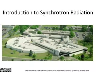
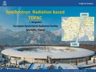
Synchrotron Radiation Facilities. Alessandro G. Ruggiero Brookhaven National Laboratory CINVESTAV, Mexico City, January, 24-26, 2007. World Radiation Facilities. There are 60 SR Facilities in the World listed at http://www.camd.lsu.edu/lightsourcefacilities.html SPring - 8 Hyogo, Japan

Synchrotron Radiation Facilities
E N D
Presentation Transcript
Synchrotron Radiation Facilities Alessandro G. Ruggiero Brookhaven National Laboratory CINVESTAV, Mexico City, January, 24-26, 2007
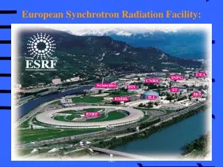
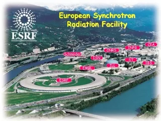
World Radiation Facilities • There are 60 SR Facilities in the World listed at • http://www.camd.lsu.edu/lightsourcefacilities.html • SPring - 8 Hyogo, Japan • Advanced Photon Source Argonne, IL, United States • European Synchrotron Radiation Facility Grenoble, France • National Synchrotron Light Source Brookhaven, NY, United States Alessandro G. Ruggiero Brookhaven National Laboratory
3rd-Generation Facilities and Brookhaven Number of Periods Alessandro G. Ruggiero Brookhaven National Laboratory
Linac Booster Storage Ring Beam Lines Typical SR Facility Undulator - Wiggler e-Source Insertion Devices Bending Magnet Energy, E Circumference, 2πR No. of Periods, M Beam Current, I Bending Radius, Number of Beam Lines Alessandro G. Ruggiero Brookhaven National Laboratory
a2 = H + ()2b2 = V = E/E = π a a Quadrupoles Dipoles Alessandro G. Ruggiero Brookhaven National Laboratory
F B D B F Lattice Design Period • x m11 m12 0 0 0 m16 x • x' m21 m22 0 0 0 m26 x' • y 0 0 m33 m34 0 0 y • y' 0 0 m43 m44 0 0 y' • s -m26 -m16 0 0 1 m56 s • 2 0 0 0 0 0 1 1 Equations of Motion x radial and y vertical displacement from reference orbit x’, y’ are angles that electron trajectory makes with reference orbit. ’ d / ds s longitudinal coordinate x'’ + KH(s) x = h(s) h(s) = curvature = 1 / = E/E y'’ + KV(s) x = 0 KH,V(s) = focusing function = G/ B Drift LengthL 1 L 0 0 0 0 0 1 0 0 0 0 0 0 1 L 0 0 0 0 0 1 0 0 0 0 0 0 1 0 0 0 0 0 0 1 Total Period Matrix M H or V cos + sinsin … … -sin cos – sin … … … … … … … … H = Np/2π Dipole Bending AngleRadius cos sin 0 0 0 (1- cos) --1sin cos 0 0 0 sin 0 0 1 0 0 0 0 0 1 0 0 sin(1- cos) 0 0 1 ( - sin) 0 0 0 0 0 1 QuadrupoleK = (G/B)1/2Length L Strength = LK cosK-1sin 0 0 0 0 -Ksin cos 0 0 0 0 0 0 coshK-1sinh0 0 0 0 Ksinh cosh0 0 0 0 0 0 1 0 0 0 0 0 0 1 For QF Invert 2x2 H with 2x2 V for QD betatron ’ dispersion H V tunes c momentum compaction factor = Magnet Errors & Misallignment -- H-V Coupling Chromaticity d H,V / d -- Sextupoles -- Non-linearities Alessandro G. Ruggiero Brookhaven National Laboratory
Lattice Functions Alessandro G. Ruggiero Brookhaven National Laboratory
Lattice Functions Alessandro G. Ruggiero Brookhaven National Laboratory
Radiation Integrals • I1 = ds / all integrals are over Dipoles • I2 = ds / 2 • I3 = ds / |3| • I4 = (1-2n) ds / 3 n = - ( / B) dB / dx (Field Index) • I5 = H ds / |3| H = [2 + ( ' - ' / 2)] / (horizontal) • Momentum Compaction c = (E / C) dC / dE = I1 / C • Energy Loss per Turn U0 = 2re E4 I2 / 3 (mc2)3 • Damping Partition Factors JH = 1 - I4 / I2 and JE = 2 + I4 / I2 • Energy Spread E2 = (55/32√3) (h / mc) (E/mc2)2 I3 / (2 I2 + I4) • Emittance = (55/32√3) (h / mc) (E/mc2)2 I5 (I2 - I4) • = F(H, lattice) E2[GeV] / JH NDipoles • > 7.84 mm-mrad • Damping Times i [ms] = C[m] [m] / 13.2 Ji E3 [GeV] • E.D. Courant and H.S. Snyder, “Theory of Alternating Gradient Synchrotron”, Annals of Physics, 3, 1-48 (1958) • M. Sands, “The Physics of Electron Storage Rings. An Introduction”, SLAC-121, Nov.ember 1970 Alessandro G. Ruggiero Brookhaven National Laboratory
P() c Synchrotron Radiation from a Dipole Magnet • Critical Photon Energy c = h c = 3 h c 3 / 2 • c [keV] = 0.665 B[T] E2 [GeV] • c [Ao] = 18.64 / B[T] E2 [GeV] • dN / d = (photons spectral and angular distribution) • (3 6 / 4 π2) y2 (2 + -2)2 [ K2/32() + K1/32() 2 / (2 + -2) ] (I / e) / • / = vertical / horizontal opening angle • = y (1 + 2 2)3/2 / 2 • y = c / = / c • At = 0 dN / d = 1.325 x 10¹⁶ E2[GeV] I[Amp] y2K2/32(y/2) / • photons/sec/mrad/mrad • Integrating over dN / d = 2.457 x 10¹⁶ E[GeV] I[Amp] y (∫y∞K5/3(x)dx) / • photons/sec/mrad • dP/d [mW/mrad] = 8.73 x 10³ E4[GeV] I[Amp] y2 (∫y∞K5/3(x)dx) / [m] • Total Power PT[kW] = U0[keV] I[Amp] = 88.5 E4[GeV] I[Amp] / [m] • J. Schwinger, Phys. Rev. 97, 470 (1955) Alessandro G. Ruggiero Brookhaven National Laboratory
RF Acceleration • Because of the energy loss U0 to Synchrotron Radiation, the Beam is continuously • re-accelerated with a RF system of cavities at the frequency fRF and peak voltageVRF • The revolution Frequency f0 = c / C ( =1) • The Harmonic Number h = fRF / f0 • The Synchronous Phase s = arcsin [1/q] • q = eVRF / U0 • The RF acceptance RF = ± [2 U0 [(q2 - 1)1/2 - arccos (1/q)] / π c h E]1/2 • Synchrotron Tune s = fs / f0 = [eVRFc h cos s / 2π E]1/2 • rms Bunch Length L = c cE/ 2 π fs Alessandro G. Ruggiero Brookhaven National Laboratory
b a Abet Vacuum Chamber and Beam Cross-Section ARF RF Bucket and e-Bunch Beam Lifetime • Gas Scattering (elastic) • 1/scat = 4re2Z2π d c [<H>Hmax / a2 + <V>Vmax / b2] / 2 2 • Bremstrahlung • 1/brem = (16/411)re2Z2 d c ln[183 Z-1/3][-ln ARF - 5/8] • Touschek • 1/T = √π re2 c N C() / H' 3 (Aacc)2 V V = 8π3/2H V L Aacc < Abet or ARF • C() = -3 e- / 2 + ∫∞ e-u ln u du / 2 u + (3 - ln + 2) ∫∞ e-u du / u • = (Aacc / H')2 • Quantum Lifetime • q = E e / 2 = ARF2/ 2E2 Alessandro G. Ruggiero Brookhaven National Laboratory
Damping Time75 msLifetime180 min Number of RF Buckets 1560 Number of Bunches 1280 Alessandro G. Ruggiero Brookhaven National Laboratory
Helical Undulator • Field Configuration (NU is the number of periods) • B = Bu[cos(kuz) x + sin(kuz) y] kU = 2π / U • Radiated WavelengthWiggler Parameter • () = U(1 + K2 + 22) / 2 2K = eBU / mckU < 1 • Spectral and Angular Distribution ( = 0) photons/sec/steradian • dN / d = 2 NU22K2 (I/e) (sin x / x)2 ( /) / (1 + K2)2 • Resonance and Width x = πNU( - r) / r • r = 2 c kU 2 / (1 + K2) /r = 1 / NU Alessandro G. Ruggiero Brookhaven National Laboratory
Planar Undulator (1) • Field Configuration (NU is the number of periods) • B = Bucos(kuz) y kU = 2π / U • Radiated WavelengthUndulator Parameter • n() = U(1 + K2/2 + 22) / 2n2K = eBU / mckU < 1 • Spectral and Angular Distribution ( = 0) photons/sec/steradian • dN / d = NU22 Fn(K) (I/e) (sin xn / xn)2 ( /) • Resonance and Width xn = πNUn( - n) / n • n = 2 nc kU 2 / (1 + K2/2) n /n = 1 / nNU Alessandro G. Ruggiero Brookhaven National Laboratory
Planar Undulator (2) • Form Factor • Fn(K) = [nK / (1 + K2/2)]2 [J(n+1)/2 (u) - J(n-1)/2 (u) ]2 • n = 1, 3, 5, …. u = n K2/(4 + 2K2) • Total Power Radiated • PT[W] = 7.26 E2[GeV] I[Amp] NUK2 / U[cm] Alessandro G. Ruggiero Brookhaven National Laboratory
Planar Wiggler • The Insertion is a Wiggler when K >> 1 (with NW periods) • Critical Energy • c() = c0 [1 - ( / K)2]1/2 • c0[keV] = 0.665 B[T] E2[GeV] • K = 0.934 B[T] w[cm] • Flux = 2 NW x equivalent arc source flux of same c • Total Power Radiated • PT[W] = 7.26 E2[GeV] I[Amp] NWK2 / W[cm] Alessandro G. Ruggiero Brookhaven National Laboratory
Klystron AC - to -RF Conversion Efficiency ~ 50-60 % Alessandro G. Ruggiero Brookhaven National Laboratory
Free Electron Laser (1) • The FEL has three components: • - e-beam with E and I -> P = E x I • a fraction of the beam power is converted to FEL power • - Undulator (Helical) with BU and U • stimulates radiation at wavelength cc = U(1 + K2) / 2 2 • - Low-Level e.m. Field at c (beam noise, external input, mirrors,….) • creates beam self-bunching at lengths comparable to c • Electron Orbit in Undulator K = eBU / mckUkU = 2π / U • = (K / )[ cos(kUz) x – sin(kUz) y ] + 0z • 0 = [1 – (1 + K2) / 2]1/2 A Coherent Source of Tunable Radiation If e-Bunch length >> c then Prad ~ N If e-Bunch length <~ c then Prad ~ N2 Alessandro G. Ruggiero Brookhaven National Laboratory
Free Electron Laser (2) • Plane wave propagating along the Undulator axis k = 2π / • E = E0 [ cos(kz - t + ) x + sin(kz - t + ) y ] • Energy TransferPonderomotive Force Phase • mc2 d / dt = ec E0 (K / ) sin ( + ) = (k + kU) z – t + 0 • Synchronism Condition d / dt = 0 -> = c • Otherwise d / dt = k (z / 0 – 1) -> … bunching ... • Synchronous Particle mc2 ds / dt = ec E0 (K / s) sins • Other Particle mc2 d / dt = ec E0 (K / ) sin Alessandro G. Ruggiero Brookhaven National Laboratory
/B s = 0 30o 45o 60o s = 90o Free Electron Laser (3) Energy Difference = mc2 ( – s) Equations of Motion d / dt = eE0 c (K / ) (sin – sins) d / dt = ckU / mc2 3 Hamiltonian H = eE0 c (K / ) (cos + sins) + ckU 2 / 2mc2 3 Bucket Height B = 2e mc2E0K 2 / kU Phase Oscillation Frequency = eE0K kU cos s / m 4 Alessandro G. Ruggiero Brookhaven National Laboratory
FEL Amplification • Small-Signal Gain (Meady’s Formula) • (few %) Undulator Length < Gain Length • G = 4 √2 π cK2 (I/ IA) NW3 [ d(sinx / x)2 / dx] / W2 (1 + K2)3/2 • 17 kA (Alfven current)x = π NW /radiation cross-section • High-Gain • (single pass) Undulator Length > Gain Length FEL Volume Length • Stored Energy WFEL = E02 VFEL / 4π • Power Gain d WFEL / dt = 0.633 kW E2[GeV] I[A] BU[T] LU[m] Alessandro G. Ruggiero Brookhaven National Laboratory
FEL Performance Evaluation (Low Gain) • Plane Undulator • Length LU = NUU • Number of Periods NU • Period Length U • Field Strength BU • Undulator Parameter K = 0.934 BU[T] U[cm] • Radiated Wavelength c = 0.13 x 10⁻⁶ U (1 + K2/2) / E2[GeV] • Radiated Power PT[kW] = 0.633 E2[GeV] I[Amp] BU2[T] LU[m] • BU = 1 T 10 T • U = 1 cm • E = 1 GeV 3 GeV • I = 1 Amp • LU = 1 m 15 m • c = 19 Ao • PT = 0.633 kW • PBeam = 1 GW Eff[%] = 0.633 x10⁻⁴ E[GeV] BU2[T] LU[m] = 0.3 Alessandro G. Ruggiero Brookhaven National Laboratory
Which Accelerator? Alessandro G. Ruggiero Brookhaven National Laboratory
Procedure • -Talk to the User’s Community • -Determine Requirements: • Wavelength, c • Flux dN / d • Number of Beam Lines • -Chose Accelerator Type E, I, C, Lattice,… • -Plan in Phases: • SR from Bending Magnets alone • Insertion Devices • FEL • -Cost and Schedule Estimate Alessandro G. Ruggiero Brookhaven National Laboratory
Performance • c [Ao] = 18.64 / B[T] E2 [GeV] • dN / d [ph/Amp sec mrad 0.1% BW] = 1.6 x 10¹³ E[GeV] at = c • For instance with B = 1.25 T -> c [Ao] = 15 / E2 [GeV] Alessandro G. Ruggiero Brookhaven National Laboratory
Circumference, Beam Current and RF Power • U0 =Energy Loss / Turn • Isomagnetic Storage Ring • Packing Factor = Bending Radius / Average RadiusR = 0.20 • rms Energy Spread = E / E = (Cq 2 / JE )1/2 Cq = 3.84 x 10⁻¹³ m Alessandro G. Ruggiero Brookhaven National Laboratory
Brightness and Beam Emittance • Flux dN / d = photons / Amp sec sterorad 0.1% BW • Brightness dN / ddS = photons / Amp sec sterorad mm2 0.1% BW • Beam Emittance = H2 / L = (JE / JH) (E / E)2 < H >Mag • Lattice Choice (Horizontal Plane, Isomagnet Storage Ring) • < H >Mag = ∫Mag { 2 + (L ' – L' / 2 )2 } ds / 2π L • ≈ c R / H • To increase Brightness -> reduce beam spot size H -> reduce Emittance -> choose Low-Dispersion Lattice Alessandro G. Ruggiero Brookhaven National Laboratory
Facilities Comparison L, Horizantal ~ 1 m 10% coupling Alessandro G. Ruggiero Brookhaven National Laboratory
Brightness -- Spring-8 & APS Alessandro G. Ruggiero Brookhaven National Laboratory
Brightness -- ESRF Alessandro G. Ruggiero Brookhaven National Laboratory
Brightness -- NSLS Alessandro G. Ruggiero Brookhaven National Laboratory
Damping and Quantum Fluctuation = emittance or energy spread • d / dt = – / + DQ = 0 • Equilibrium ∞ = DQ • It takes 3 or 4 Damping • Times to reach • Equilibrium. • Usually • initial > ∞ > source / ∞ ∞ t / Alessandro G. Ruggiero Brookhaven National Laboratory