Synchrotron radiation
600 likes | 646 Vues
This lecture summary covers the impact of synchrotron radiation on electron beam dynamics, including radiation damping, quantum excitation, RF cavity interaction, and stability considerations above and below transition. Longitudinal motion equations and the RF bucket concept are discussed, emphasizing the role of energy deviation and time delay. The computation of radiation damping in the longitudinal plane is detailed, with a focus on the dependence of energy loss per turn on particle energy. The derivation of longitudinal damping time through power radiated calculations is described, incorporating dispersion function and energy deviation considerations.

Synchrotron radiation
E N D
Presentation Transcript
Synchrotron radiation R. Bartolini John Adams Institute for Accelerator Science, University of Oxford and Diamond Light Source JUAS 2018 Week 4 - 2018
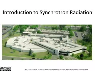
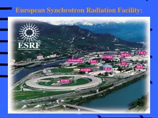
Contents Introduction to synchrotron radiation properties of synchrotron radiation synchrotron light sources angular distribution of power radiated by accelerated particles angular and frequency distribution of energy radiated: radiation from undulators and wigglers Beam dynamics with synchrotron radiation electron beam dynamics in storage rings radiation damping and radiation excitation emittance and brilliance low emittance lattices diffraction limited storage rings short introduction to free electron lasers (FELs)
The electrons radiate energy: the equations of motion have a dissipative term; the system is non conservative and Liouville’s theorem does not apply; The emission of radiation leads to damping of the betatron and synchrotron oscillations Radiation is not emitted continuously but in individual photons. The energy emitted is a random variable with a known distribution (from the theory of synchrotron radiation seen in previous lectures) This randomness introduce fluctuations which tend to increase the betatron and synchrotron oscillations Damping and growth reach an equilibrium in an electron synchrotron. This equilibrium defines the characteristics of the electron beam (e.g. emittance, energy spread, bunch size, etc) Effects of synchrotron radiation on electron beam dynamics
We will now look at the effect of radiation damping on the three planes of motion We will use two equivalent formalisms: damping from the equations of motion in phase space damping as a change in the Courant-Snyder invariant The system is non-conservative hence the Courant-Snyder invariant – i.e. the area of the ellipse in phase space, is no longer a constant of motion We will then consider the effect of radiation quantum excitation on the three planes of motion We will use the formalism of the change of the Courant-Snyder invariant Effects of synchrotron radiation on electron beam dynamics
A particle in an RF cavity changes energy according to the phase of the RF field found in the cavity From the lecture on longitudinal motion On the other hand, a particle lose energy because of synchrotron radiation, interaction with the vacuum pipe, etc. Assume that for each turn the energy losses are U0 The synchronous particle is the particle that arrives at the RF cavity when the voltage is such that it compensate exactly the average energy losses U0 Negative RF slope ensure stability for > 0 (above transition) Veksler 1944 MacMillan 1945: the principle of phase stability We describe the longitudinal dynamics in terms of the variables (, ) energy deviation w.r.t the synchronous particle and time delay w.r.t. the synchronous particle
Equations for the RF bucket RF buckets recap. > 0 above transition < 0 below transition Aide-memoire for stable motion: above transition the head goes up in energy, below transition the head goes down in energy Linearised equations for the motion in the RF bucket: the phase space trajectories become ellipses angular synchrotron frequency
In presence of synchrotron radiation losses, with energy loss per turn U0, the RF fields will compensate the loss per turn and the synchronous phase will be such that Radiation damping: Longitudinal plane (I) The energy loss per turn U0 depends on energy E. The rate of change of the energy will be given by two terms Assuming E << E and << T0 we can expand additional term responsible for damping
The derivative is responsible for the damping of the longitudinal oscillations Radiation damping: Longitudinal plane (II) Combining the two equations for (, ) in a single second order differential equation angular synchrotron frequency longitudinal damping time
We have to compute the dependence of U0 on energy the E (or rather on the energy deviation ) Computation of dU0/dE The energy loss per turn is the integral of the power radiated over the time spent in the bendings. Both depend on the energy of the particle. The time that an off-energy particle spends in the bending element dl is given by off-energy orbit This is an elementary geometric consideration on the arc length of the trajectory for different energies
Computation of dU0/dE Using the dispersion function Computing the derivative w.r.t. at = 0 we get [Sands] To compute dP/d we use the result obtained in the lecture on synchrotron radiation, whereby the instantaneous power emitted in a bending magnet with field B by a particle with energy E is given by Watch out! There is an implicit dependence of or B on E. Off energy particles have different curvatures or can experience different B if B varies with x
Computation of dU0/dE and since P is proportional to E2B2 we can write [Sands] check this as an exercise ! we get and using We have the final result
The longitudinal damping time reads Radiation damping: Longitudinal plane (III) depends only on the magnetic lattice; typically it is a small positive quantity is approximately the time it takes an electron to radiate all its energy (with constant energy loss U0 per turn) For separated function magnets with constant dipole field:
Consider a storage ring with a synchrotron tune of 0.0037 (273 turns); and a radiation damping of 6000 turns: start ¼ of synch period ½ of synch period 1 synch period Tracking example: longitudinal plane 10 synch periods 50 synch periods After 50 synchrotron periods (2 radiation damping time) the longitudinal phase space distribution has almost reached the equilibrium and is matched to the RF bucket
Consider a storage ring with a synchrotron tune of 0.0037 (273 turns); negligible radiation damping: start ¼ of synch period ½ of synch period 1 synch period Tracking example: longitudinal plane 10 synch periods 50 synch periods After 50 synchrotron periods the longitudinal phase space distribution is completely filamented (decoherence). Any injection mismatch will blow up the beam
Transverse plane: vertical oscillations (I) We assume to simplify the calculations that we are in a section of the ring where (z = 0), then We now want to investigate the radiation damping in the vertical plane. Because of radiation emission the motion in phase space is no longer conservative and symplectic, i.e. the area of the ellipse defining the Courant-Snyder invariant is changing along one turn. We want to investigate this change. The ellipse in the vertical phase space is upright. The Courant-Snyder invariant reads
Effect of the emission of a photon: The photon is emitted in the direction of the momentum of the electron (remember the cone aperture is 1/) The momentum p is changed in modulus by dp but it is not changed in direction neither z nor z’ change and the oscillation pattern is not affected since Dz = 0 (see later case where Dx 0 as for the horizontal plane) Transverse plane: vertical oscillations (II) Therefore the Courant-Snyder invariant does not change as result of the emission of a photon … however the RF cavity must replenish the energy lost by the electron
In the RF cavity the particle sees a longitudinal accelerating field therefore only the longitudinal component is increased to restore the energy Transverse plane: vertical oscillations (III) The momentum variation is no longer parallel to the momentum this leads to a reduction of the betatron oscillations amplitude The angle changes because acquired in the RF cavity
After the passage in the RF cavity the expression for the vertical invariant becomes Transverse plane: vertical oscillations (IV) The change in the Courant-Snyder invariant depends on the angle z’ for this particular electron. Let us consider now all the electrons in the phase space travelling on the ellipse, and therefore having all the same invariant A For each different z’ the change in the invariant will be different. However averaging over the electron phases, assuming a uniform distribution along the ellipse, we have and therefore The average invariant decreases.
Let us consider now all the photons emitted in one turn. The total energy lost is The RF will replenish all the energy lost in one turn. Summing the contributions , we find that in one turn: Transverse plane: vertical oscillations (V) we write The average invariant decreases exponentially with a damping time z z half of longitudinal damping time always dependent on 1/3. This derivation remains true for more general distribution of electron in phase space with invariant A (e.g Gaussian) The synchrotron radiation emission combined with the compensation of the energy loss with the RF cavity causes the damping.
Transverse plane: vertical oscillations (VI) Since the emittance of a bunch of particles is given by the average of the square of the betatron amplitude of the particles in the bunch taken ofver the bunch distribution in phase space The betatron oscillations are damped in presence of synchrotron radiation the emittance decays with a time constant which is half the radiation damping time
The damping of the horizontal oscillation can be treated with the same formalism used for the vertical plane, e.g. • consider the electron travelling on an ellipse in phase space with invariant A • compute the change in coordinates due to the emission of one photon • compute the change of coordinates due to the passage in the RF • averaging over all electron with the same invariant • compute the change in the average invariant for all photons emitted in one turn The new and fundamental difference is that in the horizontal plane we do not neglect the dispersion, i.e. Dx 0 The reference orbit changes when a quantum is emitted because of Dx in the bendings. The electron will oscillate around its new off-energy orbit. In details: Transverse plane: horizontal oscillations (I)
After the emission of a photon, the physical position and the angle of the electron do not change. However they must be referenced to a new orbit: This is the off-energy orbit corresponding to the new energy of the electron With respect to the off-energy orbit, the emission of a photon appears as an offset (and an angle) x = 0, x’ = 0 but x + xd= 0 (and likewise x’ + x’d= 0) Transverse plane: horizontal oscillations (II)
Transverse plane: horizontal oscillations (III) Invariant in the horizontal plane After the photon emission position and angle do not change but with respect to the new (off energy) orbit We follow the same line as done for the vertical plane. The equations of motion in the horizontal plane (x = 0) are and we have said that and similarly The new invariant in the horizontal plane (with respect to the new orbit) reads
The change in the Courant-Snyder invariant due to x and x’ to first order in reads Transverse plane: horizontal oscillations (IV) As before the change in the Courant Snyder invariant depends on the specific betatron coordinates x and x’of the electron . We want to average of all possible electron in an ellipse with the same Courant- Snyder invariant and get If for each photon emission the quantity is independent on x and x’, then averaging the previous expression over the phases of the betatron oscillations would give zero. However, in the horizontal plane depends on x in two ways [Sands]
Let us compute the dependence of the energy of the photon emitted in the horizontal plane on x [Sands]. Assuming that the emission of photon is described as a continuous loss of energy (no random fluctuations in the energy of the photon emitted), we have Transverse plane: horizontal oscillations (V) both P and dt depend on the betatron coordinate of the electron And, since P B2, to the first order in x
The energy change reads Transverse plane: horizontal oscillations (V) Substituting in We get The change in the Courant-Snyder invariant depends on the position and angle x and x’’for this particular electron. Let us consider now all the electrons in the phase space travelling on the ellipse, and therefore having all the same invariant A
Transverse plane: horizontal oscillations (VI) For each different x and x’ the change in the invariant will be different. However averaging over the electron phases, assuming a uniform distribution along the ellipse, we have The average invariant can now increase or decrease depending on the sign of the previous term, i.e. depending on the lattice. Let us consider all the photons emitted in one turn. The total energy lost is Summing the contributions in one turn, we find that in one turn:
Transverse plane: horizontal oscillations (VII) The change in the horizontal average invariant due to the emission of a photon >0 gives an anti-damping term As in the vertical plane we must add the contribution due to the RF that will replenish all the energy lost. Adding the RF contribution (as before assuming Dx = 0 at the RF cavities) The average horizontal invariant decreases (or increases) exponentially with a damping time z .z half of longitudinal damping time always dependent on 1/3. This remains true for more general distribution of electron in phase space with invariant A (e.g Gaussian)
Transverse plane: horizontal oscillations (VIII) Since the emittance of a bunch of particle is given by the average of the square of the betatron amplitude of the particles in the bunch As in the vertical plane, the horizontal betatron oscillations are damped in presence of synchrotron radiation the emittance decays with a time constant which is half the radiation damping time
Jx = 1 - ; Jz = 1; J = 2 + ; Damping partition numbers (I) The Ji are called damping partition numbers, because the sum of the damping rates is constant for any (any lattice) Jx + Jz + J = 4 (Robinson theorem) The results on the radiation damping times can be summarized as Damping in all planes requires –2 < < 1 Fixed U0 and E0 one can only trasfer damping from one plane to another
Adjustment of damping rates Modification of all damping rates: Increase losses U0 Adding damping wigglers to increase U0 is done in damping rings to decrease the emittance Repartition of damping rates on different planes: Robinson wigglers: increase longitudinal damping time by decreasing the horizontal damping (reducing dU/dE) Change RF: change the orbit in quadrupoles which changes and reduces x
Example: damping rings The time it takes to reach an acceptable emittance will depend on the transverse damping time The emittance needs to be reduced by large factors in a short store time T. If the natural damping time is too long, it must be decreased. This can be achieved by introducing damping wigglers. Note that damping wigglers also generate a smaller equilibrium emittance eq. Damping rings are used in linear colliders to reduce the emittance of the colliding electron and positron beams: The emittance produced by the injectors is too high (especially for positrons beams). In presence of synchrotron radiation losses the emittance is damped according to
Using ILC parameters i = 0.01 m f = 10 nm f / i= 10–6 The natural damping time is T~ 400 ms while it is required that T/x ~ 15, i.e. a damping time x ~ 30 ms (dictated by the repetition rate of the following chain of accelerators – i.e. a collider usually) Damping wigglers reduce the damping time by increasing the energy loss per turn Example: damping rings With the ILC damping ring data E = 5 GeV, = 106 m, C = 6700 m, we have U0 = 520 keV/turn x = 2ET0/U0 = 430 ms
The damping time x has to be reduced by a factor 17 to achieve e.g. 25 ms. Damping wigglers provide the extra synchrotron radiation energy losses without changing the circumference of the ring. The energy loss of a wiggler Ew with peak field B and length L and are given by Example: damping rings or in practical units the energy loss per electron reads A total wiggler length of 220 m will provide the required damping time.
Many important properties of the stored beam in an electron synchrotron are determined by integrals taken along the whole ring: Radiation integrals In particular Energy loss per turn Damping partition numbers Damping times
Synchrotron radiation losses and RF energy replacement generate a damping of the oscillation in the three planes of motion Summary The damping times depend on the energy as 1/3 and on the magnetic lattice parameters (stronger for light particles) The damping times can be modified, but at a fixed energy losses, the sum of the damping partition number is conserved regardless of the lattice type Radiation damping combined with radiation excitation determine the equilibrium beam distribution and therefore emittance, beam size, energy spread and bunch length.
Quantum nature of synchrotron emission The radiated energy is emitted in quanta: each quantum carries an energy u = ħ; The emission process is instantaneous and the time of emission of individual quanta are statistically independent; The distribution of the energy of the emitted photons can be computed from the spectral distribution of the synchrotron radiation; The emission of a photon changes suddenly the energy of the emitting electron and perturbs the orbit inducing synchrotron and betatron oscillations. These oscillations grow until reaching an equilibrium when balanced by radiation damping Quantum excitation prevents reaching zero emittance in both planes with pure damping.
Total radiated power From the lecture on synchrotron radiation Frequency distribution of the power radiated Critical frequency Critical angle at the critical frequency
From the frequency distribution of the power radiated Energy distribution of photons emitted by synchrotron radiation (I) We can get the energy distribution of the photons emitted per second: n(u) number of photons emitted per unit time with energy in u, u+du un(u) energy of photons emitted per unit time with energy in u, u+du Energy is emitted in quanta: each quantum carries an energy u = ħ un(u) must be equal to the power radiated in the frequency range du/ħ at u/ ħ
Introducing the function F() Energy distribution of photons emitted by synchrotron radiation (II) we have Using the energy distribution of the rate of emitted photons one can compute: Total number of photons emitted per second Mean energy of photons emitted per second Mean square energy of photons emitted per second
Quantum fluctuations in energy oscillations (IV) After the emission of a photon of energy u we have The time position w.r.t. the synchronous particle does not change Let us consider again the change in the invariant for linearized synchrotron oscillations We do not discard the u2 term since it is a random variable and its average over the emission of n(u)du photons per second is not negligible anymore. Notice that now also the Courant Snyder invariant becomes a random variable!
We want to compute the average of the random variable A over the distribution of the energy of the photon emitted Quantum fluctuations in energy oscillations (II) Quantum excitation Radiation damping We have to compute the averages of u and u2 over the distribution n(u)du of number of photons emitted per second. As observed the term with the square of the photon energy (wrt to the electron energy) is not negligible anymore
Following [Sands] the excitation term can be written as Quantum fluctuations in energy oscillations (VI) and depends on the location in the ring. We must average over the position in the ring, by taking the integral over the circumference. The contribution from the term linear in u, after the average over the energy distribution of the photon emitted, and the average around the ring reads Using these expressions…
The change in the invariant averaged over the photon emission and averaged around one turn in the ring now reads Quantum fluctuations in energy oscillations (VII) The change in the invariant still depends on the energy deviation of the initial particle. We can average in phase space over a distribution of particle with the same invariant A. A will become the averaged invariant The linear term in u generates a term similar to the expression obtained with the radiative damping. We have the differential equation for the average of the longitudinal invariant
The average longitudinal invariant decreases exponentially with a damping time and reaches an equilibrium at Quantum fluctuations in energy oscillations (VIII) This remains true for more general distribution of electron in phase space with invariant A (e.g Gaussian) The variance of the energy oscillations is for a Gaussian beam is related to the Courant-Snyder invariant by
The equilibrium value for the energy spread reads Quantum fluctuations in energy oscillations (IX) For a synchrotron with separated function magnets The relative energy spread depends only on energy and the lattice (namely the curvature radius of the dipoles)
synchrotron period 200 turns; damping time 6000 turns; A tracking example Diffusion effect off Diffusion effect on
after the emission of a photon of energy u we have Quantum fluctuations in horizontal oscillations (I) and Neglecting for the moment the linear part in u, that gives the horizontal damping, the modification of the horizontal invariant reads Invariant for linearized horizontal betatron oscillations Defining the function Dispersion invariant As before we have to compute the effect on the invariant due to the emission of a photon, averaging over the photon distribution, over the betatron phases and over the location in the ring [see Sands]:
We obtain Quantum fluctuations in horizontal oscillations (II) The linear term in u averaged over the betatron phases gives the horizontal damping Combining the two contributions we have the following differential equation for the average of the invariant in the longitudinal plane