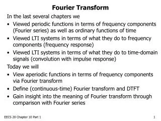
The Fourier Transform

The Fourier Transform • Last week we talked aboutconvolution as a technique for a variety of image processing applications (and we will see many more). • Convolution works in the spatial domain, i.e., it uses spatial filters that are shifted across an input image. • Sometimes it is useful to perform filtering in the frequency domaininstead. • To understand what this means and to perform such filtering, we need to take a look at the Fourier transform. Computer Vision Lecture 7: The Fourier Transform

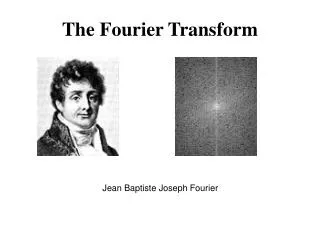
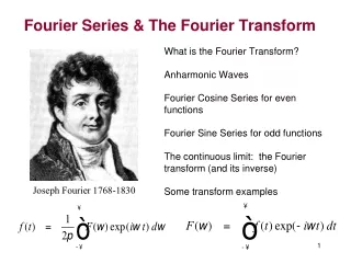
The Fourier Transform Jean Baptiste Joseph Fourier (and his Fourier-transformed image) Computer Vision Lecture 7: The Fourier Transform

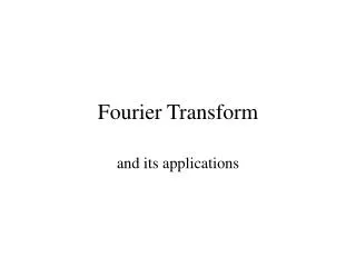
The Fourier Transform • The Fourier transform receives a function as its input and outputs another function. • The Fourier transform assumes that the input function is periodic, i.e., repetitive, and defined for all real numbers. • It transforms this function into a weighted sum of sinusoidal terms. • Let us first look at one-dimensional functions. • Later, we will move on to two-dimensional functions such as images. Computer Vision Lecture 7: The Fourier Transform

A A sin(x) 3 sin(x) B + 1 sin(3x) A+B + 0.8 sin(5x) C A+B+C + 0.4 sin(7x) D A+B+C+D Adding Sine Waves = Computer Vision Lecture 7: The Fourier Transform

The Fourier Transform • By adding a number of sine waves of different frequencies and amplitudes, we can approximate any given periodic function. • However, if we limit ourselves to only sine waves with no offset, i.e., difference in phase at x = 0, we cannot perfectly reconstruct every function. For instance, the output of our function at x = 0 must always be 0. • We could add a phase to each sine wave, but as Monsieur Fourier found out, it is sufficient to use both sine and cosine waves (which describe the same wave, but with a 90 phase difference) and keep all phases at 0. Computer Vision Lecture 7: The Fourier Transform

The Fourier Transform • So for any given function f, we could define a function Fs that assigns to any frequency an amplitude (i.e., weight) that the sine wave of that frequency will receive in our sum of sine waves. • Similarly, we could define a function Fc that does the same for the cosine waves. • In other words, these functions describe the contribution of different frequencies to the overall signal, our function f. • While f describes our function in the spatial domain (i.e., what value does it have in what position x), Fs and Fc describe the same function in the frequency domain (i.e., the extent to which different frequencies are included in the function). Computer Vision Lecture 7: The Fourier Transform

Im 1  0 0 Re Refresher: Complex Numbers • As you certainly remember, complex numbers consist of a real and an imaginary part, which we will use to represent the contribution of cosine and sine waves, respectively, to a given function. For example, 5 + 3i means Re = 5 and Im = 3. • Importantly, the exponentialfunction represents a rotation in the 2D spacespanned by the real andimaginary axes: • ei = cos  + isin  sin  cos Computer Vision Lecture 7: The Fourier Transform

The Two-Dimensional Fourier Transform Two-Dimensional Fourier Transform: Note: F(u,v) is complex, while f(x, y) is real. Two-Dimensional Inverse Fourier Transform:   amplitude basis functions and phase of required basis functions Computer Vision Lecture 7: The Fourier Transform

2D Discrete Fourier Transform (u = 0,..., N-1; v = 0,…,M-1) (x = 0,..., N-1; y = 0,…,M-1) Computer Vision Lecture 7: The Fourier Transform

2D Discrete Fourier Transform • What do these equations mean? • Well, if you look at the inverse transform, you see that each F(u, v) is multiplied by an exponential term for each pixel, and in sum they give us the original image. • In other words, each exponential function represents one particular wave, and the sum of these waves, weighted by F, is our original image f. • In the exponential term, you see an expression such as (ux + vy). This means that the variables u and v determine the “speed” with which the term increases when x and y, respectively, grow. • Since this term determines the current angle of a wave, u and v determine the frequency of the waves in horizontal and vertical direction, respectively. Computer Vision Lecture 7: The Fourier Transform

Computer Vision Lecture 7: The Fourier Transform

Magnitude And Phase Spectra • Remember that we have both Fs and Fc to describe the sine and cosine contributions, respectively, to the spatial function. • They can be used to compute the magnitude m: • … and the phase : Computer Vision Lecture 7: The Fourier Transform

Fourier Transform: Rectangle Computer Vision Lecture 7: The Fourier Transform

Fourier Transform: Spatial Shifting Computer Vision Lecture 7: The Fourier Transform

Fourier Transform: Rotation Computer Vision Lecture 7: The Fourier Transform

Fourier Transform: Multiplicity Computer Vision Lecture 7: The Fourier Transform

Fourier Transform: Real-World Images Computer Vision Lecture 7: The Fourier Transform

Fourier Transform: Low-Pass Filtering Computer Vision Lecture 7: The Fourier Transform

Fourier Transform: High-Pass Filtering Computer Vision Lecture 7: The Fourier Transform

Fourier Transform: Noise Removal Computer Vision Lecture 7: The Fourier Transform

The Fourier Transform