Download
1 / 36
360 likes | 552 Vues
Flare Ribbon Expansion and Energy Release. Ayumi Asai Nobeyama Solar Radio Observatory, NAOJ April 6, 2005 @Nainital, India. Nobeyama Radioheliograph. cadence: 1 sec spatial resolution: 10” 17 GHz / 34 GHz flare, prominence, sunspot circular polarization. http://solar.nro.nao.ac.jp/.

E N D
Flare Ribbon Expansionand Energy Release Ayumi Asai Nobeyama Solar Radio Observatory, NAOJ April 6, 2005 @Nainital, India
Nobeyama Radioheliograph • cadence: 1 sec • spatial resolution: 10” • 17 GHz / 34 GHz • flare, prominence, sunspot • circular polarization http://solar.nro.nao.ac.jp/
Flare Ribbon Expansionand Energy Release Ayumi Asai Nobeyama Solar Radio Observatory, NAOJ April 6, 2005 @Nainital, India
Magnetic Reconnection Model (Carmichael 1964; Sturrock 1966; Hirayama 1974; Kopp-Pneuman 1976) • well explains observed phenomena • phenomenologically succeeded • still needs to be checked quantitatively and qualitatively
Flare Ribbons magnetic reconnection 2001-4-10 flare (Hida Obs.) size : 104 – 105 km duration : 10 min – 10 hours Ha flare ribbons
What can we learn from Flare Ribbons? • Two elongated bright regions (two ribbon) on each side of magnetic neutral line • Two ribbons have the opposite magnetic polarity (N/S) to each other • Two ribbons separate to each other with a speed of about several 10 km/s in earlier phase, and decelerated to about several km/s in later phase • Correspond to the footpoints of post-flare loops What can we learn from flare ribbons?
2001-April-10 Flare • Flare • April 10, 2001 • 05:10 UT • GOES X2.3 NOAA 9415 West East Ha images taken with Sartorius Telescope
Observations Data Ha・・Sartorius Telescope, Kyoto University (Ha center) EUV・・TRACE (171A) HXR・・Yohkoh/HXT microwave・・ Nobeyama Radioheliograph magnetogram・・SOHO/MDI Sartorius Telescope (Kwasan Obs.)
1. Conjugacy of Ha Footpoints • Nonthermal particles and thermal conduction bombard the chromospheric plasma at both the footpoints simultaneously The temporal evolution of both the footpoints is very similar(Sakao 1994) • We identify the conjugated pairs of the footpoints which show similar light curves ? N S simultaneously brighten
Conjugacy of Ha footpoints • divided flare ribbons into fine meshes • determine “conjugated footpoints” by using cross-correlation function red:positive, blue:negative
TRACE Flare Loops TRACE 171A The TRACE loops really connect the pairs. West East
Temporal evolution of Ha kernels The pairs are classified according to the times of brightening
Focus on Each Pair Movement of the site of energy release t
2. Energy Release Rate • quantitative estimation of the amount of the released energy, based on the magnetic reconnection model and by using observable values test the reconnection model Reconnection model indicates Bc: coronal magnetic field strength vin: inflow velocity A : area of the reconnection region
Energy Release Rate Electric Field Bc: coronal magnetic field strength Bp: photospheric magnetic field strength vin: inflow velocity vf: separation speed of flare ribbons conservation of magnetic flux It is very difficult to estimate physical values (Bc, vin) in the corona Poynting Flux I estimate the energy release rate, by using observable values (Bp, vf)
Evolution of Flare Ribbons Neutral Line B v I estimate the reconnection rate vB, and the Poynting flux vB2as the representations of the energy release rates.
Evolution of Flare Ribbons Neutral Line B v I estimate the reconnection rate vB, and the Poynting flux vB2as the representations of the energy release rates.
Evolution of Flare Ribbons Neutral Line B v I estimate the reconnection rate vB, and the Poynting flux vB2as the representations of the energy release rates.
Energy Release Rate HXR sources flare ribbons Ha image Energy Release Rate We compare the derived energy release rate with HXR light curves
Reconnection Rate and Poynting Flux microwave HXR An HXR burst occurred on the slit (05:19 UT). reconnection rate Poynting flux
Reconnection Rate and Poynting Flux microwave HXR reconnection rate An HXR burst occurred on the slit (05:26 UT). Poynting flux
Quantitative Estimation W2 E2 W2 E2 W1 Comparison of Poynting and Electric Field (Reconnection Rate) between the Ha kernels with HXR sources and those without ones E1 W3 E3 W4 E4
3. Ha kernel spectroscopy Ichimoto & Kurokawa 1984 Ha spectrum • Ha line is shifted red-ward red-asymmetry • velocity : 50-100 km/s flare X-ray corona Ha compression chromosphere l Ha line
Red-Asymmetry Map • we calculated as an indicator of r.a. • all over the flare ribbon, the tendency of r.a. is seen map
Red-Asymmetry Distribution • strong asymmetry @outer edges of the flare ribbon 1000~3000 km (?) • at HXR sources, r.a. is not necessary strong
Scatter plot (intensity vs RA) • Iblue-Ired vs r.a. scatter plot • the brighter the kernel is, the stronger the r.a. is intensity of Ha kernel blue red
Summary • We can learn from Ha flare ribbons: • Select conjugated footpoints by calculating the cross-correlation function • Estimate energy release rate, by using the separation motions of two ribbons and the photospheric magnetic field strengths • Examine red-asymmetry distribution by using Ha wing data
2D / 3D observed as Ha flare ribbons
Temporal evolution of Red-Asymmetry • red-asymmetry peak precedes the HXR/microwave peaks (HXR bursts are not necessary associated with strong red-asymmetry)
Scatter Plot Haカーネルの強度 bright より明るいカーネルほど、赤でより明るい red asymmetryがより強く出ていることを示唆? dark bright in red bright in blue
Haカーネルのライトカーブ 場所によってさまざまなライトカーブを示す
Neupert Effect • The shape of light curves in HXRs and microwaves correspond to the time-derivative of SXR ones! (Neupert 1968) • Radiation in SXRs ~ total energy HXR/microwave radiations ~ energy release rate
Ha線での放射 • 非熱的粒子や熱伝導がフレアループに沿って伝播し、足元で彩層に突入する Haカーネルの増光 Haフレアリボンの形成 • エネルギー解放したループの足元の場所が分かる Haフレアリボンとして観測
Haカーネルと硬X線放射源 • フレア(磁気リコネクション)に伴い、硬X線で非熱的な放射源が生成 • 非熱的・高エネルギー粒子が彩層に突入 硬X線放射源とHaカーネルを生成 非熱的・高エネルギー粒子の彩層突入 硬X線 Ha線 コロナ 彩層 制動放射 急激な熱化など