Pumps and compressors
Pumps and compressors. Pumps and compressors. Sub-chapters 9.1. Positive-displacement pumps 9.2. Centrifugal pumps 9.3. Positive-displacement compressors 9.4. Rotary compressors 9.5. Compressor efficiency. In Chapters 4, 5, and 6, we have written energy balance equations which

Pumps and compressors
E N D
Presentation Transcript
Pumps and compressors Sub-chapters • 9.1. Positive-displacement pumps • 9.2. Centrifugal pumps • 9.3. Positive-displacement compressors • 9.4. Rotary compressors • 9.5. Compressor efficiency
In Chapters 4, 5, and 6, we have written energy balance equations which involve a dWa,o term (see Sec. 4.8 for a definition of dWa.o). • For steady-flow this term generally represents the action of a pump, fan, blower, compressor turbine, etc. • This chapter discusses the fluid mechanics of the devices which actually perform that dWa,o
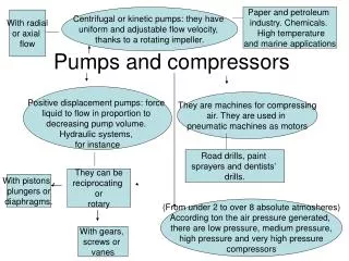
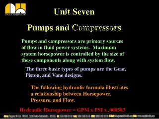
POSITIVE-DISPLACEMENT PUMPS • Pumps work on liquid and compressors work on a gas. • Most mechanical pumps are one of these: • Positive-displacement • Centrifugal • Special designs with characteristics intermediate between the two • In addition, there are nonmechanical pumps (i.e., electromagnetic, ion, diffusion,jet, etc.), which are not considered here.
Positive-displacement(PD) pumps work by allowing a fluid to flow into enclosed cavity from a low-pressuresource, trapping the fluid, and then forcing it out into a high-pressure receiver by decreasing the volume of the cavity. • Examples are the fuel and oil pumps on most automobiles, the pumps on most hydraulic systems, and the hearts most animals. • Figure 9.1 shows the cross-sectional view of a simple PD pump
The operating cycle of such a pump is as follows, starting with the piston at the top • The piston starts downward, creating a slight vacuum in the cylinder. • The pressure of the fluid in the inlet line is high enough relative to this vacuum to force open the left-hand valve, whose spring has been designed to let the valve open under this slight pressure difference. • Fluid flows in during the entire downward movement of the piston.
The piston reaches the bottom of its stroke and starts upward. This raises the pressure in the cylinder> the pressure in the inlet line, so the inlet valve is pulled shut by its spring. • When the pressure in the cylinder > the pressure in the outlet line, the outlet valve is forced open. • The piston pushes the fluid out into the outlet line. • The piston starts downward again; the spring closes the outlet valve, because the pressure in the cylinder has fallen, and the cycle begins again
Suppose that we test such a pump, using a pump test stand, as shown in Fig. 9.2. • With the pump discharge pressure regulator (a control valve) we can regulate the discharge pressure and, using the bucket, scale, and clock, determine the flow rate corresponding to that pressure. • For a given speed of the pump's motor, the results for various discharge pressures are shown in Fig 9.3.
From Fig. 9.3 we see that PD pumps are practically constant-volumetric flow-rate devices (at a fixed motor speed) and that they can generate large pressures. The danger that these large pressures will break something is so severe that these pumps must always have some kind of safety valve to relieve the pressure if a line is accidentally blocked. • For a perfect PD pump and an absolutely incompressible fluid, the volumetric flow rate equals the volume swept out per unit time by the piston, Volumetric flow rate = piston area x piston travel x cycles/time (9.1)
For an actual pump the flow rate will be slightly less because of various fluid leakages. • If we write Bernoulli's equation (Eq. 5.7) from the inlet of this pump to the outlet and solve for the work input to the pump, we find • (9.2) • The 1st term on the right represents the "useful" work done by the pump: increasing the pressure, elevation, or velocity of the • The 2nd represents the "useless" work done in heating either the fluid the surroundings.
The normal definition of pump efficiency is (9.3) • This gives in terms of a unit mass of fluid passing through the pump. • It is often convenient to multiply the top and bottom of this equation by the mass flow rate , which makes the denominator exactly equal to the power supplied to the pump: (9.4)
Example 9.1. A pump is pumping 50gal/min of water from a pressure of 30psia to a pressure of 100psia. The changes in elevation and velocity are negligible. The motor which drives the pump is supplying 2.80 hp. What is the efficiency of the pump? • The mass flow rate through the pump is
so, from Eq. 9.4, • From this calculation we see that the numerator in Eq. 9.4 has the dimension of horsepower. This numerator is often referred to as the hydraulic horsepower of the pump.
becomes equal to the hydraulic horsepower divided by the total horsepower supplied to the pump. • For large PD pumps, can be as high as 0.90; for small pumps it is less. • One may show (Prob. 9.4) that for the pump in this example the energy which was converted to friction heating and thereby heated the fluid would cause a negligible temperature rise. The same is not true of gas compressors, as discussed in Sec. 9.3.
If we connect our PD pump to a sump, as shown in Fig. 9.4, and start the motor, what will happen? A PD pump is generally operable as a vacuum pump. Therefore, the pump will create a vacuum in the inlet line. This will make the fluid rise in the inlet line. • If we write the head form of Bernoulli's equation, Eq. 5.11, between the free surface of the fluid (point 1) and the inside of the pump cylinder, there is no pump work over this section; so
. (9.5) • If, as shown in Fig. 9.4, the fluid tank is open to atmosphere, then P1 = Patm. The maximum value of h possible corresponds to P2 = 0. If there is no friction and the velocity at 2 is negligible, then • . (9.6) • For water under normal Patm and Troom, hmax 34 ft = 10 m. This height is called the suction lift.
The actual suction lift obtainable with a PD pump < that shown Eq. 9.6 because • There is always some line friction, some friction effect through the pump inlet valve, and some inlet velocity. • The pressure on the liquid cannot be reduced to zero with causing the liquid to boil. All liquids have some finite vapor pressure. For water at room temperature, it is about 0.3 psia or 0.02 atm. If the pressure < 0.02 atm, the liquid will boil.
Example 9.2. • We wish to pump 200 gal/ min of water at 150oF from a sump. We have a PD pump which can reduce absolute pressure in its cylinder to 1 psia. We have an F/g (for the pipe only) of 4 ft. The friction effect in the valve may be considered the same as that of a sudden expansion (see Sec.5.5) with the inlet velocity equal to the fluid flow velocity through the valve, which is 10 ft/s. The atmospheric pressure at this location >= 14.5 psia. • What is the maximum elevation above the water level in the sump at which we can place the pump inlet?
Answer • The lowest pressure we can allow in the cylinder P is 3.72 psia, the vapor pressure of water at 150oF. If the pressure < 3.72 psia, the water would boil, interrupting the flow. The density of water at 150oF = 61.3 lbm/ft3. • Thus • =19.8 ft = 6.04 m
CENTRIFUGAL PUMPS • A centrifugal pump raises the pressure of a liquid by giving it a high kinetic energy and then converting that kinetic energy to injection work. The water pump on most automobiles is a typical centrifugal pump. • As shown in Fig. 9.5. it consists of an impeller (i.e., a wheel with blades) and some form of housing with a central inlet and a peripheral outlet. • The fluid flows in the central inlet into the "eye" of the impeller, is spun outward by the rotating impeller, and flows out through the peripheral outlet.
To analyze such a pump on a very simplified basis, use Bernoulli's equation (Eq. 5.7) between the inlet pipe (point 1) and the outer tips of the impeller blades (point 2) • The elevation change and V1 negligible. We assume that the friction losses also are negligible. • Although P2 > P1, this term is small compared with the change in kinetic energy • (9.7)
This equation indicates that the pump work, which enters through the rotating shaft, principally increases the kinetic energy of the fluid as it flows across the impeller from the eye to the tips of the blades. • The tangential velocity at any point is tangential velocity = radius x angular velocity (9.8) • The angular velocity (2 rpm) is constant for the whole impeller, but the radius from 0 at the eye to a significant value at the tip of the blades. Max tangential vel. = V2
Use Bernoulli's equation from the tip of the blades (point 2) to the outlet pipe (point 3). • The change in elevation is negligible, and friction is neglected. No work on the fluid between points 2 and 3. V3 negligible. Thus (9.9) • This equation indicates that the section of the pump from the tip of the rotor blades to the outlet pipe converts the kinetic energy of the fluid to increased pressure
Thus, the centrifugal pump may be considered a two-stage device: 1. The impeller increases the kinetic energy of the fluid at practically constant pressure. 2. The diffuser converts this kinetic energy to increased pressure. • Equations 9.7 and 9.9 suggest that for a given pump size and speed, P/(g) should be constant. • Figure 9.6 shows the results of such a test for a large, high-efficiency pump. As predicted by the simple model, for low flow rates, P/(g) ≠ f(flowrate)
Example 9.3. A typical centrifugal pump runs at 1800rpm (mainly because of the convenient availability of 1800rpm electric motors). If the fluid being pumped is water, what is the maximum pressure difference across the pump for impeller diameters of 1, 3, and 10 in? • Using Eq 9.9 • For impeller 1 in
= 0.41 psi = 2.86 kPa • For 3-in dia impeller • For 10-in dia impeller
This example illustrates the fact that centrifugal pumps supply small +P with small impellers and high +P with large impellers. • When a large pressure rise is required, we can obtain it by hooking several centrifugal pumps in series (head to tail). • The normal practice is to put several impellers on a common shaft and to design a casing so that the outlet from one impeller is fed through a diffuser directly to the inlet of the next impeller. This is particularly true of deep-well centrifugal irrigation pump.
The performance curve of a real pump, shown on Fig. 9.6, indicates some the limitations of our simple model: • As the flow rate is large, the +P decreases, which is not predicted by the model. • The model would indicate = 100 % for all flow rates, whereas the actual varies over a wide range, peaking near 90 % at the design operating range.
As in Example 9.3, we let the pump turn at 1800 rpm and have an impeller of 10-in diameter. If the pump is full of water, the pump has a P of +42 psi; so there is no problem with the suction lift. • When we start the pump, the fluid around the impeller is air. Therefore, from Eq. 9.9 we find +P (V1 is kept constant due to tip design) is
If this pump is discharging into the atm and the sump is open to atm, then the pump, when full of air, can lift the water only a height of • To get a centrifugal pump going, one must replace the air in the system with liquid. This is called priming. • Numerous schemes for performing this function are available
Centrifugal pumps are often used to pump boiling liquids, e.g., at the bottom of many distillation columns. • Between inlet pipe (point 1) and the point on the blades of impeller where the pump starts to increase pressure (point 1a) • . (9.10) • P1a falls and boiling may occur. V1a, P1a • In this case the pump must be located far enough below the boiling surface so that the +P due to gravity from the boiling surface to the pump eye> -P in the pump eye.
This elevation is shown as h in Fig. 9.7. This distance required below the boiling surface is called the net positive suction head (NPSH).
The pressure in Fig. 9.8 is the pressure measured at the pump inlet. If there is significant frictional -P between the vessel and the pump, then h in Fig. 9.7 must be increased to overcome this additional -P.
POSITIVE-DISPLACEMENT COMPRESSORS • A compressor has Poutlet/Pinlet >> 1. • If P is small, the device is called a blower or fan. Blowers and fans work practically the way as centrifugal pumps, and their behavior can be readily predicted by equations developed for centrifugal pumps. • To compress a gas to a final (absolute) pressure > 1.1 times its inlet pressure requires a compressor, and the change in density of the gas must be taken into account.
A PD compressor has the same general form as a PD pump. The operating sequence is the same as that described in Sec. 9.1. The differences are in the size and speed of the various parts (recall Eq 9.9). • The pressure-volume history of the gas in the cylinder of such a compressor is shown in Fig. 9-9. Cycle: ABCD
The work of any single-piston process is given by • . (9.11) • The work done by the compressor on the gas is the gross work done on the gas (under curve CDA) minus the work done by the gas on the piston as the flowed in (area under curve BC); thus, the net work is the area enclosed by curve ABCD. This is the work done on the gas. • Compressors are often used to compress gases which can be reasonably well represented by the perfect-gas law PV= nRT.
If a compressor works slowly enough and has good cooling facilities, then the gas in the cylinder will be at practically a constant temp throughout the entire compression process. Then we may substitute nRT/P for V in Eq. 9.12 and integrate: • . (9.13)
However, in most compressors the piston moves too rapidly for the gas to be cooled much by the cylinder walls. • If so, the gas will undergo what is practically a reversible, adiabatic process, i.e., an isentropic process. • .PVk = P1V1k = constant [adiabatic] (9.14) • Inserting this in Eq. 9.11 • . • . (9.15)
Example 9.4. A 100 % efficient compressor is required to compress from 1 to 3 atm. The inlet temperature is 68oF. Calculate the work pound-mole for an isothermal compressor and an adiabatic compressor. • For an isothermal compressor, • For an adiabatic compressor
Equations 9.13 and 9.15 in Example 9.4 indicate that the required work for an adiabatic compressor is always > that for an isothermal compressor with the same inlet and outlet pressures. • Therefore, it is advantageous to try to make real compressors as nearly isothermal as possible. • One way to do this is to cool the cylinders of the compressor, and this is generally done with cooling jackets or cooling fins on compressors. • Another way is by staging and intercooling; see Example 9.5
Example 9.5. Air is to be compressed from 1 to 10 atm. The inlet temp is 68oF. What is the work per mole for (a) an isothermal compressor, (b) an adiabatic compressor, and (c) a two-stage adiabatic compressor in which the gas is compressed adiabatically to 3 atm, then cooled to 68oF, and then compressed from 3 to 10 atm? • For an isothermal compressor,
For an adiabatic compressor, • For a two-stage adiabatic compressor, =2862 Btu/lbmol=6.66 kJ/mol.
This example illustrates the advantage of staging and intercooling. • With an infinite number of stageswith intercooling, an adiabatic compressor would have the same performance as an isothermal compressor (Prob. 9.21). • Thus, the behavior of an isothermal compressor represents the best performance obtainable by staging. • The optimum number of stages is found by an economic balance between the extra cost of each additional stage and the improved performance as the number of stages is increased. • Large PD compressors typically have stage Pout/Pin of 3-5 and of 75- 85% (Sec. 9.5)