Chapter 5: Traffic Stream Characteristics
Chapter 5: Traffic Stream Characteristics. Chapter objectives: By the end of this chapter the student will be able to:. Explain the difference between uninterrupted flow and interrupted flow Explain the three principal traffic-stream parameters and how to obtain them

Chapter 5: Traffic Stream Characteristics
E N D
Presentation Transcript
Chapter 5: Traffic Stream Characteristics Chapter objectives: By the end of this chapter the student will be able to: • Explain the difference between uninterrupted flow and interrupted flow • Explain the three principal traffic-stream parameters and how to obtain them • Explain the relationship among the three macroscopic principal traffic-stream parameters Chapter 5
5.1 Types of traffic facilities Remember it does not mean the quality of operation. Chapter 5
5.2 Traffic stream parameters Chapter 5
5.2.1 Volume and flow rate What’s the difference between “Volume” and “Flow (or Flow rate)”? • Sub-hourly volume and flow rate • Define PHF = (peak hourly volume) / (max. rate of flow for that hour) • PHF = V/(4 * V15) • What does this tell you? • v = V/PHF • = peak flow rate for the 15-minute peak period • Can you define these? • AADT • AAWT • ADT • AWT • DDHV = AADT * K * D (Review Tables 5.1 and 5.2 & 5.3 queuing) Chapter 5
Illustration of Daily Volume Parameters Prob 5-4 is similar to this one. Chapter 5
Hourly Volumes DDHV=ADT*K*D Chapter 5
Subhourly Volume and Rates of Flow If capacity is 4,200 vph, then the 15-min capacity volume is 4,200/4 = 1,050. Chapter 5
Peak Hour Factor, PHF Chapter 5
Example: Prob. 5-6 Chapter 5
5.2.2 Speed and travel time Time mean and space mean speed: Know the difference? Every 2 seconds vehicles arrive at Chapter 5 (See page 101 and Table 5.5)
Illustrative Computation of TMS and SMS Chapter 5
5.2.3 Density and occupancy Definition: the number of vehicles occupying a given length of highway or lane (vpm, vpmpl, v/km, v/km/lane) Unit length (1 mile or 1 km) Relationship among v, S, D: v = S * D Flow rate = Speed * Density Chapter 5
Occupancy as a surrogate parameter for density • Density is difficult to measure. So, we use “occupancy” as a surrogate measure for density. This can be obtained by traffic detectors of any kind. • Occupancy: the percent of the roadway (in terms of time) that is covered (occupied) by vehicles. Apparent occupancy Actual occupancy This is the occupancy measured at a point. Chapter 5
Flow rate, speed and occupancy are given; estimate density Typically occupancies given by the detectors are apparent occupancies. (Eq.5-7) But if average flow rate and average speed for a certain time period are given, density can be computed as: Chapter 5
Derivation of the Density-Occupancy Relationship • Estimate SMS using detector data • Compute total time occupied (not occupancy) by N vehicles detected in time period T • Solve the first equation for average time occupied by each vehicle • Plug in the 3rdeq into 2ndeq • Compute the occupancy Oapp. N/T turned out to be flow rate, q. Also q/SMS is density by definition. Now the relation between occupancy, Oapp, and density, D, was established. • Solve for D. Voila, you get Eq. 5.7. Chapter 5
Spacing or Space headway Headway or Time headway 5.2.4 Spacing and Headway: Microscopic Parameters These are in English units. D (Density) = 5280 / da where da is average spacing v (Flow rate) = 3600 / ha where ha is average headway S (Average speed) = da / ha Chapter 5
5.3 Relationships among flow rate, speed, and density Do you remember whose flow model is used for this? S = Sf –(Sf/Dj)*D v = S*D = [Sf –(Sf/Dj)*D] *D Flow (v) Density (D)
5.3 Relationships among flow rate, speed, and density (2) Do you remember whose flow model is used for this? S = Sf –(Sf/Dj)*D Mean free speed Optimal flow or capacity Unstable flow area Optimal speed Flow (v) Speed is the slope. S = v/D Uncongested flow Congested flow Optimal (critical) density Jam density Density (D)
Beck St. NB Work Zone Entry Area, Chapter 5