Summarizing and Displaying Data

1. Summarizing and Displaying Data Chapter 2

2. Goals for Chapter 2 • To illustrate: • A summary of numerical data is more easily comprehended than the list itself • To explain: • the shape of the distribution of numerical data; terms used to describe this shape. • To learn: • how to construct stem-and-leaf plots, histograms; numerical values to summarize data • center of data distribution: mean, median, mode • variability of data distribution: range, interquartile range, standard deviation • To discuss: • what kinds of summaries are best for various measurements

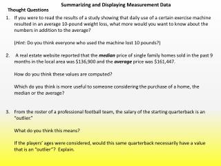
3. Thought Question 1: • Salaries of male and female employees are being compared to see if discrimination exists. • How would you present the data ?

4. Thought Question 2: • Suppose you are comparing two job offers and one of your considerations is the cost of living in each area. You get the local newspapers and record the price of 50 advertised apartments for each community. • How would you summarize the rent values for each community in order to make a useful comparison?

5. Thought Question 3: • Your boss wants to find out whether your company spends appreciably more on direct mail advertising than other companies of the same size in the industry. • What data would you present and how?

6. Thought Question 4: • Your boss wants to find out whether there is a direct relation between gross annual sales and annual expenditures for direct mail advertising for companies like yours. • What data would you present and how?

7. Types of Data • Qualitative--”Categorical” • Answer “Yes” or “No”; “Male” or “Female”; “Sick” or “Healthy”; hair color. • Quantitative--”Measurement” • Discrete (integer values): counting, ordering • Continuous (example): height, weight,

8. Three Properties of a Set of Data (Distribution): • 1. The center location • described by mean, median or mode • 2. The variability • described by range, interquartile range (IQR), standard deviation • 3. The shape • symmetric (the same on either side of the center--mean, median and mode are the same value) • skewed (different on one side of center, mean different from mode different from median)

9. Definitions for Center (Location) • Mean: average of values: • xmean= xbar = ( xi) / N, where values of xi go over all N values in sample. • Median: Value of xi that is in the middle of the ordered values: • xmedian = x(N+1)/2 if N is odd; • xmedian = (xN/2 + xN/2+1 )/2 if N is even; • Mode: most frequent value

10. Measures of Variability • Range: difference between minimum and maximum values: • range = xN - x1 • Interquartile Range (IQR): contains 50% of values (25% below median, 25% above). • IQR= Q3 - Q1 • Q1 is first quartile value; Q3 is third quartile value • Variance: measure of average square variation from mean; • Standard Deviation: square root of variance.

11. Example--Ex02.11: Production Data. • Production per shift (maximum is 720 cars /shift): • 688, 711, 625, 701, 688, 667, 694, 630, 547, 703, 688, 697, 703, 656, 677, 700, 702, 688, 691, 664, 688, 679, 708, 699, 667. • Production values--ordered • 547, 625, 630, 656, 664, 667, 667, 679, 688, 688, 688, 688, 688, 691, 694, 697, 699, 700, 701, 702, 703, 703, 703, 708, 711

12. Example--Ex02.11: Production Data-2. • Stem -and-leaf diagram of Production Data Leaf Unit = 10, N=26 1 5 4 1 5 1 5 1 6 3 6 23 4 6 5 9 6 66677 (9) 6 888889999 8 7 00000001

13. Example--Ex02.11: Production Data-3. Leaf Unit = 10, N=26 1 5 4 1 5 1 5 1 6 3 6 23 4 6 5 9 6 66677 (9) 6 888889999 8 7 00000001 MEDIAN: 68x (688); Q1: 66x (667); Q3: 70x (701); 25% of the values (6.5) are below Q1, 25% above Q3; 50% of the values are below the median, 50% above.

14. Production Data--Boxplot Edges of box are at Q1 and Q3; whiskers extend 1.5*std.dev from edges or until max or min value; note outlier (“*”)