Understanding Earth Science Data with Interactive 3D Visualization
Understanding Earth Science Data with Interactive 3D Visualization. Alan Norton and John Clyne NCAR/CISL Tutorial at Korean Supercomputing October 12, 2012.


Understanding Earth Science Data with Interactive 3D Visualization
E N D
Presentation Transcript
Understanding Earth Science Data with Interactive 3D Visualization Alan Norton and John Clyne NCAR/CISL Tutorial at Korean Supercomputing October 12, 2012 This work is funded in part through U.S. National Science Foundation grants 03-25934 and 09-06379, and through a TeraGrid GIG award, and with support from the Korean Institute for Science and Technology Information (KISTI) vapor@ucar.edu
Tutorial Overview Purpose : Demonstrate the use of VAPOR in interactively visualizing and animating earth science data Utilizing VAPOR (A visualization and analysis package developed at NCAR): We shall demonstrate many of the useful capabilities of VAPOR, as applied to weather, ocean, and other models Example data is provided so that you can repeat the visualizations on your own computer, by following the instructions in these PowerPoint slides. Attendees are not expected to perform these visualizations during the tutorial! Please ask questions whenever you don’t understand what is being shown! vapor@ucar.edu
Tutorial Outline (Intro) • Intro to VAPOR • VAPOR Overview • Requirements • Installation • How to run vapor GUI • Vapor GUI organization • User Help • Data provided with this tutorial • How to obtain georeferenced images vapor@ucar.edu
Tutorial Outline: Typhoon Jangmi Exercise • Set up a visualization session in VAPOR using a simulation of Typhoon Jangmi (Sept. 2008) • Applygeo-referenced image to terrain • Volume rendering: Visualize the typhoon progress with QCLOUD • Build a Transfer Function (color/opacity map) • Create derived variables using Python • Visualize Isosurfaces of wind speed • Color isosurface with another variable • Capture an animation sequence vapor@ucar.edu
Tutorial Outline: Typhoon Jangmi concluded • Using the vapor_wrf Python module to visualize radar reflectivity • Visualize 2D variables, e.g. 2D radar reflectivity • Barbs: show wind direction • Flow Images: Animate the flow in planar cross-section • Flow integration (wind visualization) • Streamlines: observe how the air flows through the typhoon • Use the Probe to visualize a vertical slice of W • Use the Probe to place flow seed points, based on vertical wind speed vapor@ucar.edu
Tutorial Outline: Additional topics • Unsteady flow: • ERICA example video (M. Shapiro) VAPOR features new in version 2.2: • Animation control of J. Coen’s fire simulation • Visualize MOM data (global and regional examples) • Visualize ROMS example vapor@ucar.edu
VAPOR overview The VAPOR project is intended to address the problem of understanding data that is too big to interactively read or write • VAPOR is the Visualization and Analysis Platform for Oceanic, atmospheric and solar Research • Goal: Enable scientists to interactively analyze and visualize massive datasets resulting from fluid dynamics simulation • Narrow Domain focus: 2D and 3D, gridded, time-varying turbulence datasets, especially earth-science simulation output. • Model-specific support: WRF-ARW; soon: MOM, POP, ROMS • Essential features: • Wavelet data representation for accelerated data access • Exploits GPU for fast rendering • Designed to be used by earth scientists, not visualization engineers. • Available (free) on Mac, Windows, Linux Alan Norton (vapor@ucar.edu)
VAPOR Requirements • Runs on Linux, Windows, Mac workstations • 1GB of memory is sufficient (more is better) • Requires a modern graphics card • Recent nVidia and AMD cards work well. Some Intel cards are OK. • May be necessary to update graphics drivers to get full functionality • 3-button mouse needed for 3D navigation • Need sufficient disk space to hold the data to be visualized vapor@ucar.edu
VAPOR Installation • Download free binary installer (Vapor 2.1) from “Downloads” menu on VAPOR website http://www.vapor.ucar.edu • VAPOR is available for Linux, Mac, and Windows • Registration is required • You may need Administrative privileges on your computer • Source is usually not needed • Installation instructions for each platform are provided under the “Documentation” menu, including “User Environment Setup” on Mac and Linux. vapor@ucar.edu
Launching the VAPOR GUI • Click on the VAPOR icon • or from a shell, issue the command “vaporgui” vapor@ucar.edu
VAPOR GUI window organization • Menus: File, Edit, Data, Capture, Help • Top: A few commonly used buttons and selectors • Right-hand side: One or more 3D Visualization windows • Left-hand side: Tabs to control visualization and other properties: • DVR, Flow, Iso, Probe, Image, 2D, Region, View, Animation, Model, Barbs • From Edit Menu you can launch: • Visualizer Features Panel • User Preferences Panel • Python Script Editor vapor@ucar.edu
VAPOR GUI features vapor@ucar.edu
User help Tooltips are available for most functions in the tabs: Hold the mouse over the element in the tab More detailed context-sensitive help: From Help Menu, click “? Explain This”, then click in the GUI. On the VAPOR Website (http://www.vapor.ucar.edu), click on the “Documentation” menu for explanations of most functions Several tutorials are available in the “Training” menu on the VAPOR Website VAPOR Forum is available under the “Support” menu for online discussion. E-mail us at vapor@ucar.edu for questions or problems vapor@ucar.edu
Setup User Preferences From Edit menu, click “Edit User Preferences” Set Cache Size (Megabytes) to the amount of memory you expect to have available (e.g. the physical memory on your workstation) Many other user preferences can be set, e.g. background color, default directories, etc. Click OK, and save preferences (if you want to have them always set) vapor@ucar.edu
WRF Data provided for this tutorial • Low-resolution version of Typhoon Jangmi (will download quickly): • VAPOR dataset in Jangmi_lowres.zipcan be downloaded from: ftp://ftp.ucar.edu/vapor/data/jangmi_lowres.zip • jangmi_lowres.vdf VAPOR metadata file • jangmi_lowres_data/ : directory of VAPOR data • Jangmi_terrain.tif : terrain image • Contains everything needed for this tutorial, but at lowered resolution. • Full typhoon Jangmi WRF output files (not necessary): • Download: ftp://ftp.ucar.edu/vapor/data/jangmiWrfout1.zip , ftp://ftp.ucar.edu/vapor/data/jangmiWrfout2.zip • 60 wrfout files, will be slow to download • May be used for highest quality visualization • Unzip these to a directory for use with this tutorial vapor@ucar.edu
Obtaining images to use with VAPOR • Geo-referenced satellite images can be retrieved from the Web, and VAPOR will insert them at the correct world coordinates. • VAPOR provides a shell script “getWMSImage.sh” that can be used to retrieve Web Mapping Service images for a specified longitude/latitude rectangle. It is however somewhat intermittent because of instability of the NASA Web Mapping Service. • A geo-tiff terrain image for the typhoon data has been provided in the jangmi_lowres.zip file. • Several useful images are pre-installed with VAPOR, including a world-wide terrain image, and political boundaries of the U.S and the world. Apply these by clicking “Select Installed Image” in the Image panel. vapor@ucar.edu
Set-up to visualize a WRF dataset (1) • Launch ‘vaporgui’ (Desktop Icon: ) • From Data menu: “Import WRF-ARW output files into current session”: select all (60) jangmiwrfout* files to import vapor@ucar.edu
Data reduction needed? If you did not download the entire set of 60 wrfout files, you can still use a much smaller Vapor Data Collection (VDC) for this tutorial. The jangmi_lowres.vdf file (and the associated directory jangmi_lowres_data) is a resolution-reduced version of the variables needed for this tutorial. Instead of using the “Import WRF-ARW files” capability, use “load a dataset into current session” and specify the jangmi_lowres.vdf file. vapor@ucar.edu
Set-up to visualize a WRF dataset (2) • From Edit menu, click “Edit Visualizer Features” then: • Stretch Z by factor of 20, press <enter> to confirm value • Specify time annotation, “Date/Time stamp” • Click “OK” vapor@ucar.edu
Set-up to visualize a WRF dataset (3) • To include a terrain image: Click on the “Image” tab • Click “Select Image File” and choose “jangmi_terrain.tif” • Check “Apply image to terrain” • Check the “Instance: 1” checkbox at the top of the Image tab to view the terrain image. vapor@ucar.edu
Ways to Control the 3D Scene • To navigate: Rotate, Zoom in, Translate by dragging in the scene with left, right and middle mouse buttons. • Click “Home” icon ( ) to return to starting viewpoint • Click “Eye” icon ( ) to see full domain • Use Edit→Undo if you make a mistake • Use the VCR controls at the top left of the window to animate through time (see where the WRF d02 domain is positioned over time) • When you type in values, be sure to press <enter> to confirm the values. vapor@ucar.edu
Navigation tools in VAPOR GUI vapor@ucar.edu
Volume Visualization of QCLOUD • Using VCR control, type in time step 34, press enter. • Click the “wheel” icon ( ) to set navigation mode • Select DVR panel (direct volume rendering) • Select variable “QCLOUD” (cloud water mixing ratio) • Check “Instance:1” to enable volume rendering • Note: May need to click “Fit Data” to get correct bounds on Mac vapor@ucar.edu
Volume Visualization: Edit Transfer function (1) • Click “Histo” to see histogram of data values of QCLOUD at current timestep • To make the clouds white, set 4 color control points to white • Either select/edit with right mouse button, or • Select point and then choose white color in color selector. vapor@ucar.edu
Volume Visualization: Edit Transfer function (2) • To edit the transparency: • Drag the 2nd control point down to make the lower values more transparent • Use slider on the right to control overall transparency. • Click the play button “►” to animate the clouds associated with the typhoon. vapor@ucar.edu
Visualization of typhoon: QCLOUD at time step 42 vapor@ucar.edu
Define derived variable • From VAPOR Edit menu, choose “Edit Python Program defining a new variable” • In the Python editor: • Check U, V, and W as Input 3D Variables. • Add “Wind” as Output 3D Variable. • Type in the one-line python script: Wind = sqrt(U*U+V*V+W*W) 4. Click “Test”; if response is “Successful Test” it’s OK; then click “Apply” vapor@ucar.edu
Isosurfaces of Wind (1) • In the Iso tab: • Select variable “Wind” • Check “Instance:1” to enable • Set histo right bound to 70, then “Fit to View” and “Histo” to see Wind histogram • Set the isovalue near 30 (use slider or type it in) • In the DVR tab: disable DVR (un-check Instance: 1) • Using VCR control: • Set current time step to 44 • Click on Iso tab vapor@ucar.edu
Isosurfaces of Wind (2) To color the isosurface of Wind by QRAIN (or other variable): • Scroll down in the Iso tab to the transfer function, under Appearance • Set the mapped variable to “QRAIN”. • Click the button “Load Installed TF” below the transfer function, and load “reversedOpaque.vtf”. This makes low values violet-blue, high values orange-red. • Set the right domain bound of the transfer function to 0.001, so that the large values of QRAIN will show up as red in the isosurface. • Animate from time step 20 to see the typhoon vortex pass over Taiwan • Enable the DVR to combine clouds, wind and rain in one visualization. vapor@ucar.edu
Capture an animation sequence Save a sequence of jpeg files of your visualization: • Set the time step to 0 • From Capture menu, choose “Begin image capture sequence…” • Choose a jpeg file name in a directory where you can write files. • Click the play ( ) button. • When animation is done, from the Capture menu, click “End flow capture sequence” • (Use Quicktime Pro, ffmpeg, etc. to convert to movie file.) See jangmi.mov in images directory vapor@ucar.edu
Use VAPOR/WRF python support Vapor includes Python routines for weather analysis, such as radar reflectivity, sea-level pressure, cloud-top temperature, potential vorticity… (Documented on the VAPOR Website under “Data analysis with VAPOR”) • Disable the DVR and the Isosurface. Set time step = 30. • Write a Python script to create a new variable “dbz” which represents the simulated radar reflectivity. The python script consists of the two lines: import vapor_wrf dbz = vapor_wrf.DBZ(P,PB,QRAIN,0,QSNOW,T,QVAPOR) • Specify that dbz is an output 3D variable • Specify that P, PB, QRAIN, QSNOW, T, and QVAPOR are input 3D variables. • Visualize the DVR of dbz (click Fit Data and click “fit to view”) • Reduce opacity slider to its center position • Compare this with rain, by creating an isosurface of QRAIN=5.e-05, set the isosurface color to be Constant (white). isosurface to have vapor@ucar.edu
Radar reflectivity with isosurface of QRAINas Typhoon Jangmi approaches Taiwan vapor@ucar.edu
Calculate 2D Radar Reflectivity • Disable the Iso and the DVR. • Write a Python script to create a new variable “dbz2d”which represents the vertical max radar reflectivity. The python script consists of the two lines: import vapor_wrf dbz2d=vapor_wrf.DBZ_MAX(P,PB,QRAIN,0,QSNOW,T,QVAPOR) • Specify that dbz2d is an output 2D variable • Specify that P, PB, QRAIN, QSNOW, T, and QVAPOR are input 3D variables. • Click “Test” and then “Apply” vapor@ucar.edu
Visualize 2D Radar Reflectivity Disable the DVR and the ISO renderers Select 2D tab, choose “dbz2d” as variable Click “Fit Data” , “Fit to View” and “Histo” buttons for the 2D transfer function editor. Slide the leftmost control point down to the bottom so that zero reflectivity will display as transparent. Enable the 2D visualizer (check Instance: 1) Set the z coordinate of the 2D plane to 500 (just above the surface) Enable the ISO visualizer, set its Opacity to 0.5, so you can compare the rain to the radar in the planar image vapor@ucar.edu
2D Radar Reflectivity with QRAIN isosurface vapor@ucar.edu
Flow Visualization Overview • Flow direction can be illustrated using the Barbs tab. • Flow can be illustrated in cross-section using the flow image capability in the Probe tab. • Vapor can display streamlines (steady flow, constant time) and pathlines (unsteady flow, showing particle paths over time) • Streamlines and path lines are established by seed points (starting points for flow integration) • Seed points can be: • Random: Randomly placed within a range of x, y, and z values, or • Nonrandom: Evenly spaced in x, y, and z dimensions, or • Seed List: Explicitly placed in the scene • Vapor Rake tool is provided to specify a box for random or evenly spaced (nonrandom) seeds (looks like: ) • VAPOR Probe tool ( ) can be used to position flow seed points. vapor@ucar.edu
Display wind barbs Disable the ISO and the 2D renderer Click on the “Barbs” tab at the far left of the tabs Enable the Barbs (you should see arrows spiraling around the typhoon Under Layout Options, check “Offset vertical position by terrain height”, and set the X and Y grid dimensions to 20 Under Appearance options, set the Barb thickness to 1.5 and the scale factor to 1500 Enable the DVR of QCLOUD (retain previous DVR settings) Animate. vapor@ucar.edu
Wind Barbs with QCLOUD vapor@ucar.edu
Flow images Flow can be visualized in planar cross-section using the “Flow Image” capability in the Probe. Disable the Barbs and the DVR. Click on the Probe arrow( ) in the Mode settings. In the Probe tab, set Probe Type to “Flow Image” Under Probe Layout options, click “Fit to Region” Grab the middle handle of the probe with the right mouse and drag it down near the ocean (say 1000m) Enable the probe Animate the flow in the Probe Image settings by clicking the “Play” button “►” Note the vortex location at frames 42-44 using probe cursor vapor@ucar.edu
Flow image of Jangmi in horizontal plane vapor@ucar.edu
Random streamlines (1) • Disable Probe • Click on Flow tab • Set time step to 45 • In flow tab, select U, V, W as steady field variables. • Check “Instance: 1” to enable steady flow (streamlines). Ignore the warning message. • Click “Show Flow Seeding Settings” • Specify seed count 100 (random) for steady flow, press <enter> to set the value. • Under Appearance settings, adjust smoothness (~300) and diameter (~0.3) vapor@ucar.edu
Random streamlines (2), using Rake • Select flow rake ( at top left, Mode selector). Note box and handles. • Grab the top handle of the rake with the right mouse button, pull it down about 1/3 of the way down (the flow seeds will be nearer the ground.) • Using the right mouse button, shrink the rake to a smaller box enclosing the eye of the typhoon • Color flow lines according to “position on flow” (in Appearance settings) See how the wind is drawn in at ground level and climbs through the eyewall fig12.vss vapor@ucar.edu
Use the probe to see a vertical slice of W (1) Probe is useful to investigate the wind flow near the eye of the typhoon, by placing seed points where the W field is strongest • Disable the flow (uncheck Instance:1 box in Flow tab) • Set the time step to 36 • Select Probe mode( ) in the Mode selector at the top. Select Probe Type to Data Value • Enable probe (check Instance:1 box in Probe tab) • Set the Probe variable to “W” vapor@ucar.edu
Using the probe to see a vertical slice of W (2) To view a vertical slice through the typhoon: Under “Probe Layout options”: • Click 90 degree rotate • Select “+X” to get a vertical slice. • Click “Fit to Region” button In Appearance Parameters at the bottom of the probe panel: • Set the TF domain bounds to -0.5 and 0.5 • Click “Fit to view” and “Histo” to see the values of W in the probe vapor@ucar.edu
Cross section of typhoon (Probe of W) Viewed from the south vapor@ucar.edu
Using the probe to specify flow seed points (1) Click on the Flow tab Under Appearance Settings, set Typical Flow Length = 3 On the flow tab, under “flow seeding settings”, select “List of Seeds” instead of “Random Rake”. Check “Instance:1” to enable the flow. Ignore the warning messages (there are no seeds in the list). vapor@ucar.edu
Using the probe to specify flow seed points (2) • Click on the probe tab. • Scroll down to the probe image settings, where you see an image of the cross-section of the data • Check “Attach point to flow seed”. You should see a streamline associated with a seed point at the cursor position. • Click mouse in the image, at positions with large (purple) W values, and see the streamlines associated with the eye wall. • Click “Add Point to Flow Seeds” for streamlines that you want to keep. With 10-15 flow seeds you can visualize the wind flow pattern near the eye wall. vapor@ucar.edu
Streamlines placed with the probe vapor@ucar.edu
Unsteady Flow VAPOR also supports visualization of pathlines (particle traces). Users can visualize the trajectories massless particles would follow (forwards or backwards in time). ERICA IOP simulation was an intense Atlantic marine cyclone occurring in January 1989, as powerful as a Category 3 or 4 hurricane. Mel Shapiro and Ryan Maue provided the data which is visualized in VAPOR: Instructions for visualizing unsteady flow in VAPOR are provided in the tutorials on the VAPOR website, especially the “Georgia Weather Case Study” and the “Vapor Quick Start Guide” vapor@ucar.edu
Animation Control • A new feature in VAPOR 2.2 (not yet released) • Permits users to create animations where the viewpoint and the data time step are controlled by the user. • User specifies a sequence of keyframe viewpoints, VAPOR interpolates between them. • Example: Esperanza fire simulation, Janice Coen, NCAR • Camera is animated during the simulation to enable users to see most important details of a wildfire. vapor@ucar.edu