Download
1 / 33
330 likes | 436 Vues
CASE 2014 Technical Presentation Cycle Time and Throughput Models of Clustered Photolithography Tools for Fab-Level Simulation. Kyungsu Park and James. R. Morrison Department of Industrial and Systems Engineering KAIST, South Korea. Presentation Overview. Motivation

E N D
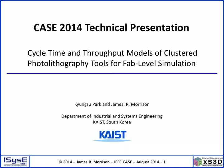
CASE 2014 Technical PresentationCycle Time and Throughput Models of Clustered Photolithography Tools for Fab-Level Simulation Kyungsu Park and James. R. Morrison Department of Industrial and Systems Engineering KAIST, South Korea
Presentation Overview • Motivation • System description: Clustered photolithography tool (CPT) • Equipment models • Linear model • Affine model • Exit recursion model • Flow line model • Numerical experiments • Same sample & same parameter • Different sample & same parameter • Different sample & different parameter • Concluding remarks
Motivation (1) • Semiconductor manufacturing • Global revenue in 2013: NT$ 9,540 billion (US$ 318 billion) • Construction costs • 300 mm wafer fab: NT$150 billion (US$ 5 billion [2]) • 450 mm wafer fab: NT$300-450 billion (US$10-15 billion) • Significant value for improvements • 1996-1999: Fab production control method earned Samsung NT$ 15 billion (US$ 1 billion [3]) additional revenue • 2005: IBM’s 30 independent supply chains merged into a single global system and saved NT$ 180 billion (US$ 6 billion [4]) • … [1]
Motivation (2) • Clustered photolithography tools (CPT) • Purchase cost of NT$ 0.6-3 billion (US$ 20-100 M [5]) • The most expensive tool in a fabricator • Typically the bottleneck of the fabricator • Key yield and cycle time contributor [5]
Motivation (3) • Want: Models for CPTs • Accurate: Predict throughput with less than 1% error • Expressive: Incorporate fundamental behaviors • Computationally tractable: Very quick to calculate results • For the purpose of: • Understanding toolset performance • Enabling capacity optimization • Toolset scheduling or optimization • Improving the quality of fab simulation models
System Description: CPT (1) Scanner Clustered Photolithography Tool • Multi-cluster tool, robot in each cluster, IF buffers, STK buffer • Scanner is often the CPT bottleneck • Largely deterministic process times • Process time can vary by product • Setups between lots (reticle changes, pre-scan setup, …) • Wafer handling robot decision policy & deadlock prevention [6]
System Description: Performance Metrics • Notation al:Arrival time of lot l to the tool Sl: Start time of lot lin the tool Cl: Completion time of lot lfrom the tool • Performance measures Cycle time of lot l: CTl:= Cl - al Lot residency time of lot l: LRTl := Cl - Sl Throughput time of lot l:TTl:= min{ LRTl, Cl – Cl-1} Computation time TT1 TT2 TT3 Lot 1 Lot 2 Lot 3 Time
Models for CPTs • Models with various levels of detail Detailed Model “Everything” Linear Model A(k1) A(k1), B Affine Models A(k1), B(k1) Access Big Data A(k1), B(k1, k2) Parametric flow lines Flow Line Models Data Analytics Empirical flow lines With complete tool log data Exit Recursion Models Simulate models With wafer in/out log data With lot in/out log data
Linear Model • Referred to as the Ax equipment model or linear model • Time between wafer completions: Al • Process time estimation: TlPT = Ak1 ∙ w(l) ( w(l): the number of wafers of lot l ) Ax Model for lot cycle time in a one machine tool Wafers enter Wafers exit m Al • Pros: • Simple to understand • Fast computation • Cons: • Exactly matched to single wafer tool, not to CPT Complete Model: l= max{ al, l-1 } l = l l = l + Ak1 ∙ w(l) l= l
Affine Models • Referred to as the Ax+Bmodel • First wafer delay: Bl • Time between wafer completions: Al • Process time estimation: TlPT = Ak1∙ (w(l) – 1) + Bl( w(l) : the number of wafers of lot l ) B can be generalized to B(k1), B(k1, k2) • Pros: • Simple to understand • Fast computation • Cons: • Only one module per process, so not matched to CPT • New lots enter only when the tool is empty Complete model: l= max{ al, l-1 } l = l l = l + B + Ak1 ∙ (w(l) - 1) l= l
Flow Line Models: Elementary Evolution Equations • Notation • aw: Arrival time of wafer wto the tool, awaw-1 • Xi(w): Entry time of wafer w into process i of the tool • : Deterministic process time for process i • Elementary Evolution Equations (EEEs) • X1(w) = max{aw , X2(w-1) } • Xi+1(w) = max{Xi(w) + , Xi+2(w-1) } • XM(w) = max{XM-1(w) + , XM(w-1) + } (M is the last process) Process i W W-1
Flow Line Models: Extensions • Elementary Evolution Equations (EEEs) can be generalized to allow: • Different classes of wafer to be produced • Multiple modules per process • Consider robotic workload in process times of modules • Consider setups – reticle setup, pre-scan setup • Parameter extraction • Parametric flow line model – Known process times, robot times, and setup times • Empirical flow line model – Parameters extracted from tool processing data Wafers enter Wafers exit
Flow Line Models: Exit Recursions • Theorem: Exact recursion for customer completion (exit) times [7,8] • Theorem: Recursive bound for customer completion (exit) times [9] R3=3 … … P2 R1=2 RM=2 … … R2=1 P1 P2 P3 PM Customers Arrive Customers Exit … Wafer Lots Arrive Wafer Lots Exit … t1 t2 t3 tM
Exit Recursion Model (1) • Conceptually based on flow line exit recursions • Complete model NoContention at bottleneck Contention at bottleneck
Exit Recursion Model (2) • Parameter extraction • Populations used as a function of available category of data
Model Properties • Proposition: Exactness on completion times in the exit recursion model • Proposition: Exactness of completion times in the linear model • Proposition: Exactness of completion times in the affine model Completion times in the exit recursion model exactly match those in a deterministic flow line from which the parameters are derived with A single class of wafers and constant setup between wafers , or Multiple wafer classes with no setup, proportional service and geometric decay within channels All completion times in the linear model exactly match those in a single process deterministic flow line from which the parameters are derived.. Throughput time can be exactly achieved on average in a flow line with different structure.. Completion times in the affine model exactly match those in a deterministic flow line in which each lot starts on an empty tool (via full flush constraint) from which the parameters are derived. Throughput time can be exactly achieved on average in a flow line with different structure..
Numerical Experiments • LWP(Longest waiting pair) robot policy[6]: gives optimal steady state throughput • Dead lock avoidance rule • Setup time ~ Uniform(210, 260); Reticle alignment ~ Uniform(240, 420) • 13,000 lots x 30 replications • Assume detail simulation is true operation. A : Linear Model B : Affine Model - A(k1),B C : Affine Model - A(k1),B(k1) D : Affine Model - A(k1),B(k1,k2) E : FL Model F : EFL Model G : ER Model - Tool Log H : ER Model - Wafer Log I : ER Model - Lot Log • [1]
Same Sample, Same Parameter • loading level : 0.95, train level : 3, lot size : {22, 23, 24} with probability {0.25, 0.5, 0.25}, both setups 36.36% 36.35% 36.28% 36.26% 2.74% 0.61% -2.59% 2.56% 2.34% 2.60% 3.52% 3.17% -0.09% -0.13% --51.32% -51.33% -51.33% -51.33% • Linear model & Affine models are only good in throughput time. • ER models & Flow line models are good in all times. 0.00% -0.00 -0.00 -0.00 -0.01% -0.02% 0.00% 0.03% -0.09%
Same Sample, Same Parameter • loading level : 0.3, train level : 3, lot size : {22, 23, 24} with probability {0.25, 0.5, 0.25}, both setups 3.97% 1.71% -17.28% -17.28% -17.28% -17.28% 0.20% -0.09% 0.81% 2.16% 2.15% 2.15% 2.15% 2.27% 2.33% -0.30% -0.57% -0.04% • Linear model & Affine models are good in cycle time, and throughput time. • ER models & Flow line models are good in all times -0.00% -0.00% -0.00% -0.00% -0.13% -0.35% 0.03% 0.07% -1.82%
Different Sample, Same Parameter • loading level : 0.95, train level : 3, lot size : {22, 23, 24} with probability {0.25, 0.5, 0.25}, both setups 58.35% 43.43% 46.19% 47.40% 2.75% 0.62% -2.58% 2.77% 2.46% 4.97% -0.37% 1.24% 2.70% 2.04% -51.40% -51.31% -51.31% -51.31% • Linear model & Affine models are only good in throughput time. • ER models & Flow line models are good in all times. -0.12% 0.05% 0.05% 0.06% 0.03% 0.01% 0.01% 0.04% -0.00%
Different Sample, Same Parameter • loading level : 0.3, train level : 3, lot size : {22, 23, 24} with probability {0.25, 0.5, 0.25}, both setups 3.98% 2.23% 0.29% -0.03% 0.84% -17.22% -17.14% -17.16% -17.16% 2.30% 2.28% 2.57% 2.65% 2.52% 2.42% 0.44% -0.17% -0.35% • Linear model & Affine models are good in cycle time, and throughput time. • ER models & Flow line models are good in all times 0.09% 0.19% 0.17% 0.17% -0.16% -0.37% 0.05% 0.14% -1.46%
Different Sample, Different Parameter • From loading level : 0.95 & train level : 3, To lading level : 0.8 & train level : 1 With lot size : {22, 23, 24} with probability {0.25, 0.5, 0.25}, both setups 0.11% 0.08% 2.17% 6.36% 5.67% 20.21% 19.29% 17.67% -4.12% -5.90% 0.43% -5.09% -4.05% -0.04% -37.96% -37.89% -37.89% -37.81% • Linear model & Affine models are slightly good in cycle time, and throughput time . • ER models are good in lot residency time, and throughput time. • Only FL models are good in all times. -0.42% -5.19% -5.09% -5.09% -4.97% -0.00% -0.11% -0.04% 0.00%
Different Sample, Different Parameter • From lot size: {22, 23, 24} with {0.25, 0.5, 0.25}, to lot size: {12, 13, 14} with {0.25, 0.5, 0.25} with loading level : 0.95, train level : 3, both setups 3.56% 7.43% -59.70% -56.67% -56.68% -56.67% 1.26% 0.39% 0.38% 17.66% 16.71% -15.21% -33.18% -14.54% -15.85% 0.29% -0.64% -0.43% • Linear model & Affine models are bad in all times. • ER models are good in lot residency time, and throughput time. • Only FL models are good in all times. -0.17% -0.13% -0.16% 0.02% -3.78% -9.92% -9.92% -9.92% -16.21%
Accuracy Comparison • Errors relative to detailed model • Error of 20%+ • Error 5-20% • Error 0-5%
Concluding Remarks • CPT: Expensive & typically fab bottleneck toolset • Models for CPT throughput time, process time & cycle time • Classic models: Linear, affine • Recent models: Flow line, exit recursion • Compare: Computation and accuracy • Next directions • Improved models: Newer exit recursions, additional parameters • Implementation: Fab simulation, optimization, etc.
References • HIS iSuppli April 2011 • ElpidaMemory, Inc., available at http://www.eplida.com, • Leachman, Robert C., Jeenyoung Kang, and Vincent Lin. "SLIM: Short cycle time and low inventory in manufacturing at samsung electronics." Interfaces32.1 (2002): 61-77 • http://www.forbes.com/forbes/2003/0811/076.html • Roger H. French and V. Hoang, “Immersion Lithography: Photomask and Wafer-Level Materials,” Tran. Annual Review of Materials Research, Vol. 39, 93-126 • Hyun Joong Yoon and Doo Yong Lee, “Deadlock-free scheduling of photolithography equipment in semiconductor fabrication,” IEEE Trans. Semi. Mfg., vol. 17, no. 1, pp. 42-54, 2004 • Avi-Itzhak, B. "A sequence of service stations with arbitrary input and regular service times." Management Science 11.5 (1965): 565-571 • Friedman, Henry D. "Reduction methods for tandem queuing systems." Operations Research 13.1 (1965): 121-131 • Park, Kyungsu, and James R. Morrison. "Performance evaluation of deterministic flow lines: Redundant modules and application to semiconductor manufacturing equipment." Automation Science and Engineering (CASE), 2010 IEEE Conference on. IEEE, 2010 • Morrison, James R. "Deterministic flow lines with applications." Automation Science and Engineering, IEEE Transactions on 7.2 (2010): 228-239 • Morrison, James R. "Multiclass flow line models of semiconductor manufacturing equipment for fab-level simulation." Automation Science and Engineering, IEEE Transactions on 8.1 (2011): 81-94 Longest waiting pair: [7] Geismar, H.N.; Sriskandarajah, C.; Ramanan, N., "Increasing throughput for robotic cells with parallel Machines and multiple robots," IEEE Trans. Auto. Sci. and Eng., vol.1, no.1, pp.84,89, Jul 2004