Download

1 / 73
730 likes | 926 Vues
Ensembles of Classifiers Evgueni Smirnov. Outline. 1 Methods for Independently Constructing Ensembles 1.1 Bagging 1.2 Randomness Injection 1.3 Feature-Selection Ensembles 1.4 Error-Correcting Output Coding 2 Methods for Coordinated Construction of Ensembles 2.1Boosting 2.2 Stacking

E N D
Outline 1 Methods for Independently Constructing Ensembles 1.1 Bagging 1.2 Randomness Injection 1.3 Feature-Selection Ensembles 1.4 Error-Correcting Output Coding 2 Methods for Coordinated Construction of Ensembles 2.1Boosting 2.2 Stacking 3 Reliable Classification 3.1 Meta-Classifier Approach 3.2 Version Spaces 3 Co-Training
Ensembles of Classifiers • Basic idea is to learn a set of classifiers (experts) and to allow them to vote. • Advantage: improvement in predictive accuracy. • Disadvantage: it is difficult to understand an ensemble of classifiers.
Why do ensembles work? Dietterich(2002) showed that ensembles overcome three problems: • The Statistical Problem arises when the hypothesis space is too large for the amount of available data. Hence, there are many hypotheses with the same accuracy on the data and the learning algorithm chooses only one of them! There is a risk that the accuracy of the chosen hypothesis is low on unseen data! • The Computational Problemarises when the learning algorithm cannot guarantees finding the best hypothesis. • The Representational Problem arises when the hypothesis space does not contain any good approximation of the target class(es). The statistical problem and computational problem result in the variance component of the error of the classifiers! The representational problem results in the bias component of the error of the classifiers!
Methods for Independently Constructing Ensembles • One way to force a learning algorithm to construct multiple hypotheses is to run the algorithm several times and provide it with somewhat different data in each run. This idea is used in the following methods: • Bagging • Randomness Injection • Feature-Selection Ensembles • Error-Correcting Output Coding.
Bagging • Employs simplest way of combining predictions that belong to the same type. • Combining can be realized with voting or averaging • Each model receives equal weight • “Idealized” version of bagging: • Sample several training sets of size n (instead of just having one training set of size n) • Build a classifier for each training set • Combine the classifier’s predictions • This improves performance in almost all cases if learning scheme is unstable (i.e. decision trees)
Bagging classifiers Classifier generation Let n be the size of the training set. For each of t iterations: Sample n instances with replacement from the training set. Apply the learning algorithm to the sample. Store the resulting classifier. classification For each of the t classifiers: Predict class of instance using classifier. Return class that was predicted most often.
Why does bagging work? • Bagging reduces variance by voting/ averaging, thus reducing the overall expected error • In the case of classification there are pathological situations where the overall error might increase • Usually, the more classifiers the better
Randomization Injection • Inject some randomization into a standard learning algorithm (usually easy): • Neural network: random initial weights • Decision tree: when splitting, choose one of the top N attributes at random (uniformly) • Dietterich (2000) showed that 200 randomized trees are statistically significantly better than C4.5 for over 33 datasets!
Feature-Selection Ensembles • Key idea: Provide a different subset of the input features in each call of the learning algorithm. • Example: Venus&Cherkauer (1996) trained an ensemble with 32 neural networks. The 32 networks were based on 8 different subsets of 119 available features and 4 different algorithms. The ensemble was significantly better than any of the neural networks!
Error-correcting output codes • Very elegant method of transforming multi-class problem into two-class problem • Simple scheme: as many binary class attributes as original classes using one-per-class coding • Idea: use error-correcting codes instead
Error-correcting output codes • Example: • What’s the true class if base classifiers predict 1011111?
Methods for Coordinated Construction of Ensembles • The key idea is to learn complementary classifiers so that instance classification is realized by taking an weighted sum of the classifiers. This idea is used in two methods: • Boosting • Stacking.
Boosting • Also uses voting/averaging but models are weighted according to their performance • Iterative procedure: new models are influenced by performance of previously built ones • New model is encouraged to become expert for instances classified incorrectly by earlier models • Intuitive justification: models should be experts that complement each other • There are several variants of this algorithm
AdaBoost.M1 classifier generation Assign equal weight to each training instance. For each of t iterations: Learn a classifier from weighted dataset. Compute error e of classifier on weighted dataset. If e equal to zero, or e greater or equal to 0.5: Terminate classifier generation. For each instance in dataset: If instance classified correctly by classifier: Multiply weight of instance by e / (1 - e). Normalize weight of all instances. classification Assign weight of zero to all classes. For each of the t classifiers: Add -log(e / (1 - e)) to weight of class predicted by the classifier. Return class with highest weight.
Remarks on Boosting • Boosting can be applied without weights using re-sampling with probability determined by weights; • Boosting decreases exponentially the training error in the number of iterations; • Boosting works well if base classifiers are not too complex and their error doesn’t become too large too quickly! • Boosting reduces the bias component of the error of simple classifiers!
Stacking • Uses metalearner instead of voting to combine predictions of base learners • Predictions of base learners (level-0 models) are used as input for meta learner (level-1 model) • Base learners usually different learning schemes • Hard to analyze theoretically: “black magic”
Stacking BC1 0 BC2 1 1 BCn BC1 BC2 BCn Class … 1 0 1 1 instance1 meta instances instance1
Stacking BC1 1 BC2 0 0 BCn BC1 BC2 BCn … 0 1 0 1 0 1 0 instance2 Class meta instances 1 instance1 instance2
Stacking BC1 BC2 BCn … 1 0 0 1 1 0 0 Meta Classifier Class meta instances 1 instance1 instance2
Stacking BC1 0 1 BC2 1 Meta Classifier 1 BCn BC1 BC2 BCn … 0 1 1 instance meta instance instance
train train test train test train test train train Meta Data test test test More on stacking • Predictions on training data can’t be used to generate data for level-1 model! The reason is that the level-0 classifier that better fit training data will be chosen by the level-1 model! Thus, • k-fold cross-validation-like scheme is employed! An example for k = 3!
More on stacking • If base learners can output probabilities it’s better to use those as input to meta learner • Which algorithm to use to generate meta learner? • In principle, any learning scheme can be applied • David Wolpert: “relatively global, smooth” model • Base learners do most of the work • Reduces risk of overfitting
Some Practical Advices • If the classifier is unstable (high variance), then apply bagging! • If the classifier is stable and simple (high bias) then apply boosting! • If the classifier is stable and complex then apply randomization injection! • If you have many classes and a binary classifier then try error-correcting codes! If it does not work then use a complex binary classifier!
Reliable Classification • Classifiers applied in critical applications with high misclassification costs need to determine whether classifications they assign to individual instances are indeed correct. • We consider two approaches that are related to ensembles of classifiers: • Meta-Classifier Approach • Version Spaces
The Task of Reliable Classification Given: • Instance space X. • Classifier space H. • Class set Y. • Training sets D X x Y. Find: • Classifier h H, h: X Y that correctly classifies future, unseen instances. If h cannot classify an instance correctly, symbol “?” is returned.
Meta Classifier Approach instance BC BC Class Meta Class instance1 0 1 0 ………………………………………….. instancen 1 1 1
Meta Classifier Approach instance BC MC Meta Class meta instances instance1 0 ………………….. instancen 1
Meta Classifier Approach Combined Classifier instance BC MC The classification of the base classifier BC is outputted if the meta classifier decides that the instance is classified correctly. Theorem.The precision of the meta classifier equals the accuracy of the combined classifier on the classified instances.
Version Spaces (Mitchell, 1978) Definition 1. Given a classifier space H and training data D, the version space VS(D) is: VS(D) = {hH | cons(h, D)}, where cons(h, D) ( (x, y) D)( y= h(x)). VS(D) H
Classification Rule of Version Spaces: the Unanimous-Voting Rule Definition 2. Given version space VS(D), instance x X receives a classification VS(D)(x) defined as follows: Definition 3. Volume V(VS(D)) of version space VS(D) is the set of all instances that are not classified by VS(D). y VS(D) ( h VS(D)) y = h(x), ? otherwise. VS(D)(x) =
Unanimous Voting VS(D) H
Unanimous Voting VS(D) H
Unanimous Voting Theorem 1. For any instance x Xandclassy Y : ( hVS(D))(h(x) = y) ( y'Y \{y}) VS(D {(x,y')})=. • Theorem 1 states the unanimous-voting rule can be implemented if we have an algorithm to test version spaces for collapse.
VS(I+, I-) H Unanimous Voting
1: Check VS(D) VS(D) H
2: Classify an instance x VS(D) x H
3: Check VS(D{(x,-)}): VS(D {(x,-)})= VS(D) x H
VS(D) , VS(D {(x,-)}) = , and VS(D {(x,+)}) imply thatx is positive VS(D) x H
2: Classify another instance x VS(D) x H
VS(D) , VS(D {(x,-)}) , and VS(D {(x,+)}) imply thatx is not classified VS(D) x H
When can we reach 100% Accuracy? • Case 1: When the data are noise-free and the classifier space Hcontains the target classifier. VS(D) H
When is it not possible to reach 100% Accuracy? • Case 2: When the classifiers space H doesnot contain the target classifier. VS(D) H
When is it not possible to reach 100% Accuracy? • Case 3: When the datasets are noisy. VS(I+, I-) H
When is it not possible to reach 100% Accuracy? • Case 3: When the datasets are noisy. VS(I+, I-) H
When is it not possible to reach 100% Accuracy? • Case 3: When the datasets are noisy. VS(I+, I-) VS(I+, I-) H
When is it not possible to reach 100% Accuracy? • Case 3: When the datasets are noisy. VS(D) H