Download

1 / 29
290 likes | 310 Vues
Explore the implications of global warming on the Northwest region with a focus on terrain and land-water contrasts. Learn about the need for local downscaling and potential surprises in weather patterns. Discover the use of dynamical downscaling and regional climate simulations to better understand the impacts of global warming.

E N D
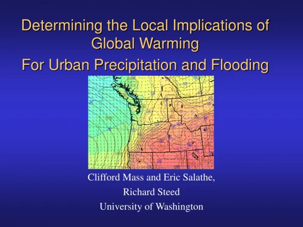
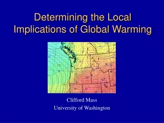
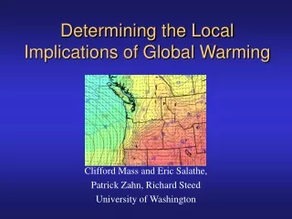
Determining the Local Implications of Global Warming Professor Clifford Mass, Eric Salathe, Patrick Zahn, Richard Steed University of Washington
Questions What are the implications of global warming for the Northwest? How will our mountains and land-water contrasts alter the story? Are we going to simply warm up or are there some potential surprises?
Regional Climate Prediction • To understand the impact of global warming on the Northwest, one starts with global circulation models (GCMs) that provide a view of the large-scale flow of the atmosphere. But GCMs can only describe features a thousand or more km in scale. • HOWEVER, Northwest weather is dominated by terrain and land-water contrasts and in order to understand the implications of global changes on our weather, local downscaling of the GCM predictions is required.
Local Northwest Weather = Terrain + Water Influence
Downscaling and Surprises • The traditional approach to use GCM output is through statistical downscaling, which finds the statistical relationship between large-scale atmospheric structures and local weather. • Statistical downscaling either assumes that current relationships will hold or makes simplifying assumptions on how local weather works.
Downscaling • Such statistical approaches may be a good start, but may give deceptive or wrong answers… there may in fact be “surprises” produced by local terrain and land/water contrasts. • In other words, the relationships between the large scale atmospheric flow and local weather might change in the future
Downscaling • There is only one way to do this right… running full weather forecasting models at high resolution over extended periods, with the large scale conditions being provided by the GCMs….called dynamical downscaling. • Such weather prediction models have all the physics, so they are capable of handling any “surprises”
Example of a Potential Surprise • Might western Washington be colder during the summer under global warming? • Reason: interior heats up, pressure falls, marine air pushes in from the ocean • Might the summers be wetter? • Why? More thunderstorms due to greater surface heating.
Downscaling • Computer power and modeling approaches are now powerful enough to make dynamical downscaling realistic… and this and the next two talks will describe work at the UW that follows this approach. • Takes advantage of the decade-long work at the UW to optimize weather prediction for our region.
UW Regional Climate Simulations • Makes use of the same weather prediction model that we have optimized for local weather prediction: the MM5. • 10-year MM5 model runs nested in the German GCM (ECHAM). • MM5 nests at 135km, 45km, and 15 km model grid spacing.
Forecast Model Nesting • 135, 45, 15 km MM5 domains • Need 15 km grid spacing to model local weather features.
Regional Modeling • Ran this configuration over several ten-year periods: • 1990-2000-to see how well the system is working • 2020-2030 and 2045-2055 (4 years so far) to view the future
Details on Current Study: GCM • Parallel Climate Model (DOE -PCM) output provide by NCAR and European ECHAM model • Horizontal resolution ~ 150km. • IPCC climate change scenario A2 -- aggressive CO2 increase (doubling by 2050) IPCC Report, 2001 IPCC Report, 2001
First things first • But to make this project a reality we needed to conquer some significant technical hurtles. • We also had to understand the biases in our coupled modeling system….so we know what is climate change and what is model bias.
Next Presentation • Patrick Zahn will tell you how we did it.
UW Regional Climate Study • We have completed the first series of simulations, having overcome a number of technical challenges. • Some early views of the results…
More Surprises? Example: More thunderstorms in summer, helping alleviate water problems--but causing more fires?
Future • We are now rerunning the regional simulations with better GCM output (ECHAM model) • Should be done in roughly 1-2 months • Will use this model output to evaluate water resources and air quality. • Will try other global warming scenarios.