Download
1 / 44
440 likes | 481 Vues
Learn about edge detection in computer vision, including models, image gradients, edge detectors, finite differences, noise effects, and optimal detector criteria.

E N D
Edge Detection T-11 Computer Vision University of Ioanina Christophoros Nikou Images and slides from: James Hayes, Brown University, Computer Vision course Svetlana Lazebnik, University of North Carolina at Chapel Hill, Computer Vision course D. Forsyth and J. Ponce. Computer Vision: A Modern Approach, Prentice Hall, 2011. R. Gonzalez and R. Woods. Digital Image Processing, Prentice Hall, 2008.
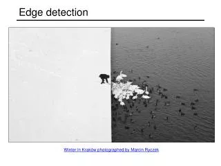
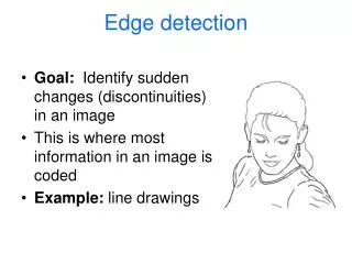
Edge detection • Goal: Identify sudden changes (discontinuities) in an image. • Intuitively, most semantic and shape information from the image can be encoded in the edges. • More compact than pixels. • Ideal: artist’s line drawing (artist also uses object-level knowledge) Source: D. Lowe
Origin of Edges • Edges are caused by a variety of factors surface normal discontinuity depth discontinuity surface color discontinuity illumination discontinuity Source: Steve Seitz
Edge model • Edge point detection • Magnitude of the first derivative. • Sign change of the second derivative. • Observations: • Second derivative produces two values for an edge (undesirable). • Its zero crossings may be used to locate the centres of thick edges.
Image gradient • The gradient of an image: The gradient points in the direction of most rapid increase in intensity The gradient direction is given by • how does this relate to the direction of the edge? The edge strength is given by the gradient magnitude Source: Steve Seitz
Recall, for 2D function, f(x,y): This is linear and shift invariant. It is therefore the result of a convolution. Approximation: which is a convolution with the mask: Differentiation and convolution Source: D. Forsyth, D. Lowe
Effect of Finite Differences on White Noise Let fbe an observed instance of the image f0 corrupted by noise w: with noise samples having mean value E[w(n)]=0 and being uncorrelated with respect to location:
Effect of Finite Differences on White Noise Applying a filter hto the degraded image: The expected value of the output is: The noise is removed in average.
Effect of Finite Differences on White Noise What happens to the standard deviation of g? Assume that a finite difference filter is used, which approximates the first derivative:
0 0 0 1 -2 1 0 0 0 Effect of Finite Differences on White Noise For a second derivative approximation: The standard deviation increases sharply! Higher order coefficients form a Pascal triangle.
Edge model and noise Intensity profile First derivative Second derivative
Edge model and noise Intensity profile First derivative Second derivative
Edge detectors respond strongly to sharp changes and noise is a sharp change. Simple finite differences are unusable. Independent additive stationary Gaussian noise is the simplest model. Noise
this model allows noise values that could be greater than maximum camera output or less than zero. for small standard deviations, this isn’t too much of a problem - it’s a fairly good model. independence may not be justified (e.g. damage to lens). may not be stationary (e.g. thermal gradients in the ccd). Issues with the Gaussian model
Why smoothing helps Smoothing (e.g. average) kernels have • Therefore, the noise standard deviation is reduced at the output, as we saw before. • Also, after smoothing (e.g. average), noise samples are no longer independent. They look like their neighbors and the derivatives are smaller.
g f * g • To find edges, look for peaks in Noisy Edge Smoothing f Source: S. Seitz
f Convolution property • Convolve with the derivative of the filter. Source: S. Seitz
Derivative of Gaussian * [1 -1] =
Derivative of Gaussian (cont.) y-direction x-direction
Tradeoff between smoothing and localization Smoothed derivative removes noise but blurs edge. It also finds edges at different “scales” affecting the semantics of the edge. σ =1 σ =3 σ =7 Source: D. Forsyth
Problems with gradient-based edge detectors σ =1 σ =2 There are three major issues: The gradient magnitude at different scales is different; which scale should we choose? The gradient magnitude is large along thick trail; how do we identify only the significant points? How do we link the relevant points up into curves?
Designing an optimal edge detector • Criteria for an “optimal” edge detector [Canny 1986]: • Good detection: the optimal detector must minimize the probability of false positives (detecting spurious edges caused by noise), as well as that of false negatives (missing real edges). • Good localization: the edges detected must be as close as possible to the true edges • Single response: the detector must return one point only for each true edge point; that is, minimize the number of local maxima around the true edge. Source: L. Fei-Fei
Canny edge detector • Probably the most widely used edge detector in computer vision. • Theoretical model: step-edges corrupted by additive Gaussian noise. • Canny has shown that the first derivative of the Gaussian closely approximates the operator that optimizes the product of signal-to-noise ratio and localization. J. Canny, A Computational Approach To Edge Detection, IEEE Trans. Pattern Analysis and Machine Intelligence, 8:679-714, 1986. Source: L. Fei-Fei
Canny edge detector (cont.) • Filter image with derivative of Gaussian. • Find magnitude and orientation of gradient. • Non-maximum suppression: • Thin multi-pixel wide “ridges” down to single pixel width. • Linking and thresholding (hysteresis): • Define two thresholds: low and high • Use the high threshold to start edge curves and the low threshold to continue them. Source: D. Lowe, L. Fei-Fei
Canny edge detector (cont.) original image
Canny edge detector (cont.) Gradient magnitude
Canny edge detector (cont.) Non-maximum suppression and hysteresis thresholding
Non-maximum suppression (cont.) We wish to mark points along the curve where the gradient magnitude is biggest. We can do this by looking for a maximum along a slice normal to the curve (non-maximum suppression). These points should form a curve. There are then two algorithmic issues: at which point is the maximum, and where is the next one? Source: D. Forsyth
Non-maximum suppression (cont.) At pixel q, we have a maximum if the value of the gradient magnitude is larger than the values at both p and at r. Interpolation provides these values. Source: D. Forsyth
Edge linking Assume the marked point is an edge point. Then we construct the tangent to the edge curve (which is normal to the gradient at that point) and use this to predict the next points (here either r or s). Source: D. Forsyth
Hysteresis Thresholding (cont.) • Use a high threshold to start edge curves and a low threshold to continue them. Source: S. Seitz
high threshold (strong edges) low threshold (weak edges) hysteresis threshold Hysteresis thresholding (cont.) Source: L. Fei-Fei
Where do humans see boundaries? human segmentation image gradient magnitude • Berkeley segmentation database:http://www.eecs.berkeley.edu/Research/Projects/CS/vision/grouping/segbench/
Learning to detect image boundaries Learn from humans which combination of features is most indicative of a “good” contour? D. Martin, C. Fowlkes and J. Malik. Learning to detect natural image boundaries using local brightness, color and texture cues. IEEE Transactions on Pattern Analysis and Machine Intelligence, Vol. 26, No 5, pp. 530-549, 2004.
What features are responsible for perceived edges? Feature profiles (oriented energy, brightness, color, and texture gradients) along the patch’s horizontal diameter D. Martin, C. Fowlkes and J. Malik. Learning to detect natural image boundaries using local brightness, color and texture cues. IEEE Transactions on Pattern Analysis and Machine Intelligence, Vol. 26, No 5, pp. 530-549, 2004.
pB Boundary Detector Figure from Fowlkes
What features are responsible for perceived edges? (cont.) D. Martin, C. Fowlkes and J. Malik. Learning to detect natural image boundaries using local brightness, color and texture cues. IEEE Transactions on Pattern Analysis and Machine Intelligence, Vol. 26, No 5, pp. 530-549, 2004.
Results Pb (0.88) Human (0.95)
Results Pb Pb (0.88) Global Pb Human (0.96) Human
Pb (0.63) Human (0.95)
Pb (0.35) Human (0.90) For more: http://www.eecs.berkeley.edu/Research/Projects/CS/vision/bsds/bench/html/108082-color.html
45 years of boundary detection Source: Arbelaez, Maire, Fowlkes, and Malik. TPAMI 2011 (pdf)