Dimensional Analysis in Fluid Phenomena
Learn how dimensional analysis establishes relationships between physical quantities in fluid dynamics. Discover its applications, principles, and reasoning for experimental work.

Dimensional Analysis in Fluid Phenomena
E N D
Presentation Transcript
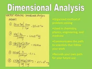
Dimensional Analysis It is a pure mathematical technique to establish a relationship between physical quantities involved in a fluid phenomenon by considering their dimensions. In dimensional analysis, from a general understanding of fluid phenomena, we first predict the physical parameters that will influence the flow, and then we group these parameters into dimensionless combinations which enable a better understanding of the flow phenomena. Dimensional analysis is particularly helpful in experimental work because it provides a guide to those things that significantly influence the phenomena; thus it indicates the direction in which experimental work should go.
Dimensional Analysis Dimensional Analysis refers to the physical nature of the quantity (Dimension) and the type of unit used to specify it. Distance has dimension L. Area has dimension L2. Volume has dimension L3. Time has dimension T. Speed has dimension L/T
Application of Dimensional Analysis • Development of an equation for fluid phenomenon • Conversion of one system of units to another • Reducing the number of variables required in an experimental program • Develop principles of hydraulic similitude for model study
Dimensional Reasoning & Homogeneity • Principle of Dimensional Homogeneity The fundamental dimensions and their respective powers should be identical on either side of the sign of equality. • Dimensional reasoning is predicated on the proposition that, for an equation to be true, then both sides of the equation must be numerically and dimensionally identical. • To take a simple example, the expression x + y = z when x =1, y =2 and z =3 is clearly numerically true but only if the dimensions of x, y and z are identical. Thus 1 elephant +2 aeroplanes =3 days is clearly nonsense but 1 metre +2 metre =3 metre is wholly accurate. An equation is only dimensionally homogeneous if all the terms have the same dimensions.
Fundamental Dimensions • We may express physical quantities in either mass-length-time (MLT) system or force-length-time (FLT) system. This is because these two systems are interrelated through Newton’s second law, which states that force equals mass times acceleration, F = ma 2nd Law of motion F = ML/T2 F = MLT-2 • Through this relation, we can covert from one system to the other. Other than convenience, it makes no difference which system we use, since the results are the same.
Dimensions of Some Common Physical Quantities [x], Length – L [m], Mass – M [t], Time – T [v], Velocity – LT-1 [a], Acceleration – LT-2 [F], Force – MLT-2 [Q], Discharge – L3T-1 [r], Mass Density – ML-3 [P], Pressure – ML-1T-2 [E], Energy – ML2T-2
Basic Concepts • All theoretical equations that relate physical quantities must be dimensionally homogeneous. That is, all the terms in an equation must have the same dimensions. For example Q = A.V (homogeneous) L3T-1 = L3T-1 • We do, however sometimes use no homogeneous equation, the best known example in fluid mechanics being the Manning equation. Mannings equation is an empirical equation. Generally the use of such equations is limited to specialized areas.
To illustrate the basic principles of dimensional analysis, let us explore the equation for the speed V with which a pressure wave travels through a fluid. We must visualize the physical problem to consider physical factors probably influence the speed. Certainly the compressibility Ev must be factor; also the density and the kinematic viscosity of the fluid might be factors. The dimensions of these quantities, written in square brackets are V=[LT-1], Ev=[FL-2]=[ML-1T-2], r=[ML-3], ν=[L2T-1] Here we converted the dimensions of Ev into the MLT system using F=[MLT-2]. Clearly, adding or subtracting such quantities will not produce dimensionally homogenous equations. We must therefore multiply them in such a way that their dimensions balance. So let us write V=C Evarbνd Where C is a dimensionless constant, and let solve for the exponents a, b, and d substituting the dimensions, we get
(LT-1)=(ML-1T-2)a (ML-3)b (L2T-1)d To satisfy dimensional homogeneity, the exponents of each dimension must be identical on both sides of this equation. Thus For M: 0 = a + b For L: 1 = -a -3b +2d For T: -1 = -2a – d Solving these three equations, we get a=1/2, b=-1/2, d=0 So that V = C √(Ev/r) This identifies basic form of the relationship, and it also determines that the wave speed is not effected by the fluid’s kinematic viscosity, ν. Dimensional analysis along such lines was developed by Lord Rayleigh.
Methods for Dimensional Analysis • Rayleigh’s Method • Buckingham’s ∏-method
Rayleigh’s Method Functional relationship between variables is expressed in the form of an exponential relation which must be dimensionally homogeneous if “y” is a function of independent variables x1,x2,x3,…..xn, then In exponential form as
Procedure Rayleigh’s Method • Write fundamental relationship of the given data • Write the same equation in exponential form • Select suitable system of fundamental dimensions • Substitute dimensions of the physical quantities • Apply dimensional homogeneity • Equate the powers and compute the values of the exponents • Substitute the values of exponents • Simplify the expression • Ideal up to three independent variables, can be used for four.
Buckingham’s ∏ method • A more generalized method of dimension analysis developed by E. Buckingham and others and is most popular now. This arranges the variables into a lesser number of dimensionless groups of variables. Because Buckingham used ∏ (pi) to represent the product of variables in each groups, we call this method Buckingham pi theorem. • “If ‘n’ is the total number of variables in a dimensionally homogenous equation containing ‘m’ fundamental dimensions, then they may be grouped into (n-m) ∏ terms. f(X1, X2, ……Xn) = 0 then the functional relationship will be written as Ф (∏1 , ∏2 ,………….∏n-m) = 0 The final equation obtained is in the form of: ∏1= f (∏2,∏3,………….∏n-m) = 0 • Suitable where n ≥ 4 • Not applicable if (n-m) = 0
Buckingham’s ∏ method Procedure • List all physical variables and note ‘n’ and ‘m’. n = Total no. of variables m = No. of fundamental dimensions (That is, [M], [L], [T]) • Compute number of ∏-terms by (n-m) • Write the equation in functional form • Write equation in general form • Select repeating variables. Must have all of the ‘m’ fundamental dimensions and should not form a ∏ among themselves • Solve each ∏-term for the unknown exponents by dimensional homogeneity.
Buckingham’s ∏ method Example: • Let us apply Buckingham’s ∏ method to an example problem that of the drag forces FD exerted on a submerged sphere as it moves through a viscous fluid. We need to follow a series of following steps when applying Buckingham’s ∏ theorem. • Step 1: Visualize the physical problem, consider the factors that are of influence and list and count the n variables. We must first consider which physical factors influence the drag force. Certainly, the size of the sphere and the velocity of the sphere must be important. The fluid properties involved are the density ρ and the viscosity μ. Thus we can write f (FD, D, V, ρ, μ) = 0 Here we used D, the sphere diameter, to represent sphere size, and f stands for “some function”. We see that n = 5. Note that the procedure cannot work if any relevant variables are omitted. Experimentation with the procedure and experience will help determine which variables are relevant.
Buckingham’s ∏ method • Step 2: Choose a dimensional system (MLT or FLT) and list the dimensions of each variables. Find m, the number of fundamental dimensions involved in all the variables. Choosing the MLT system, the dimensions are respectively MLT-2 , L , LT-1 , ML-3 , ML-1T-1 We see that M, L and T are involved in this example. So m = 3. • Step 3: Determine n-m, the number of dimensionless ∏ groups needed. In our example this is 5 – 3 = 2, so we can write Ф(∏1. ∏2) = 0 • Step 4: Form the ∏ groups by multiplying the product of the primary (repeating) variables, with unknown exponents, by each of the remaining variables, one at a time. We choose ρ, D, and V as the primary variables. Then the ∏ terms are ∏1 = Da Vbρc FD ∏2 = Da Vbρcμ-1
Buckingham’s ∏ method • Step 5: To satisfy dimensional homogeneity, equate the exponents of each dimension on both sides on each pi equation and so solve for the exponents ∏1 = Da Vbρc FD = (L)a (LT-1)b (ML-3)c (MLT-2) = M0L0T0 Equate exponents: L: a +b -3c +1 = 0 M: c +1 = 0 T: -b -2 = 0 We can solve explicitly for b = -2, c = -1, a = -2 Therefore ∏1 = D-2 V-2ρ-1 FD = FD/(ρ V2 D2)
Buckingham’s ∏ method Finally, add viscosity to D, V, and ρ to find ∏2 . Select any power you like for viscosity. By hindsight and custom, we select the power -1 to place it in the denominator ∏1 = Da Vbρcμ-1 = (L)a (LT-1)b (ML-3)c (ML-1T-1 )-1 = M0L0T0 Equate exponents: L: a +b -3c +1 = 0 M: c -1 = 0 T: -b +1 = 0 We can solve explicitly for b = 1, c = 1, a = 1 Therefore, ∏2 = D1 V1ρ1μ-1 = (D V ρ)/(μ) =R = Reynolds Number R = Reynolds Number= Ratio of inertia forces to viscous forces Check that all ∏s are in fact dimensionless
Buckingham’s ∏ method Rearrange the pi groups as desired. The pi theorem states that the ∏s are related. In this example hence FD/(ρ V2 D2) = Ф (R) So that FD = ρ V2 D2Ф (R) We must emphasize that dimensional analysis does not provide a complete solution to fluid problems. It provides a partial solution only. The success of dimensional analysis depends entirely on the ability of the individual using it to define the parameters that are applicable. If we omit an important variable. The results are incomplete, and this may lead to incorrect conclusions. Thus, to use dimensional analysis successfully, one must be familiar with the fluid phenomena involved.