Solving Problems: Intelligent Search
760 likes | 810 Vues
Explore heuristic search algorithms like Best-first Search and A* Search to efficiently solve problems by guiding the search towards the most promising solutions. Learn from expert guidance by B. John Oommen, Chancellor’s Professor at Carleton University.

Solving Problems: Intelligent Search
E N D
Presentation Transcript
Solving Problems: Intelligent Search Instructor: B. John Oommen Chancellor’s Professor Fellow: IEEE; Fellow: IAPR School of Computer Science, Carleton University, Canada The primary source of these notes are the slides of Professor Hwee Tou Ng from Singapore. I sincerely thank him for this.
Heuristic Search • Problem with DFS and BFS: No way to guide the search • Solution can be anywhere in tree. • In the worst case all possible states will be traversed • One “solution” to this problem • Probe the search space • Where is the final state likely to be • This of course will be problem specific • A function is usually created that evaluates: • How good the current solution is • This function is used to help guidethe search process • This guided search called a HeuristicSearch
A Heuristic • Derived from the Greek: heuriskein: “to find”; “to discover” • Has been used (and is sometimes still used) to mean: • “A process that may solve a given problem, but offers no guarantees of doing so” Newall, Shaw, & Simon 1963 • Heuristics can also be thought of as a “Rule of Thumb” • Can refer to any technique that improves average-case but not necessarily worst-case performance • Here: A function that provides an estimate of solution cost
Performance of Heuristics • Performance of several heuristics…
Possible Heuristics • Count the tiles out of place: • State with fewest tiles out of place is closer to the desired goal • Distance Summation: • Sum all the distance by which the tiles are out of place • State with the shortest distance is closer to the desired goal • Count reversal Tiles: • If two tiles are next to each other, and the goal requires their position to be swapped. The heuristic takes this into account by evaluating the expression (2 * number of direct tiles reversal)
Best-first Search • Idea: use an evaluation functionf(n) for each node • Estimate of “desirability” • Expand most desirable unexpanded node • Implementation: Order the nodes in fringe in decreasing order of desirability • Special cases: • Greedy best-first search • A* search
Best-first Search • Combine BFS and DFS using a heuristicfunction • Expand the branch that has the best evaluation under the heuristic function • Similar to hill climbing (move in the best direction) • But can go back to “discarded” branches
Best-first Search Algorithm • Initialize OPEN to initial state, CLOSED to Empty list • Until a Goal is found or no nodes left in Open do: • Pick the best node in OPEN • Generate its successors, place node in CLOSED • For each successor do: • If not previously generated (not found in OPEN or CLOSED) • Evaluate • Add to OPEN OPEN: Generated nodes who’s children have not been evaluated yet • Implemented as a priority queue (heap structure) CLOSED: Nodes that have been examined • Used to see if a node has been visited if searching a graph instead of a tree • Same as in DFS and BFS
F 6 F 6 D D J 1 E 4 E C A 5 C A 2 I 5 G 5 B 3 B D Closed D 1 F 6 D C A 5 E 4 C A 5 B 3 G 5 B D Closed A 8 Example of BestFS Step 3 Step 5 Step 2 Step 4 Step 1
Greedy Best-first Search • Evaluation function f(n) = h(n) (heuristic) • An estimate of cost from n to goal • hSLD(n) = straight-line distance from n to Bucharest • Greedy Best-first Search expands the node that appears to be closest to goal
Properties: Greedy Best-first Search • Complete? • No – can get stuck in loops • Iasi Neamt Iasi Neamt • Time? • O(bm) • But a good heuristic can a give dramatic improvement • Space? • O(bm) • Keeps all nodes in memory • Optimal? • No
A* Search • A modification of the Best-first Search • Used when searching for the Optimal path • Idea: Avoid expanding paths that are “expensive” • The heuristic function f(S) is broken into two parts: • Evaluation function f(n) = g(n) + h(n) • g(n) = Cost so far to reach n • h(n) = Estimated cost from n to goal • f(n) = Estimated total cost of path through n to goal
A* Algorithm • Initialize OPEN to initial state • Until a Goal is found or no nodes left in OPEN do: • Pick the best node in OPEN • Generate its successors (recording the successors in a list); • Place in CLOSED • For each successor do: • If not previously generated (not found in OPENor CLOSED) • Evaluate, add to OPEN , and record its parent • If previously generated ( found in OPENor CLOSED), and if the new path is better then the previous one • Change parent pointer that was recorded in the found node • If parent changed • Update the cost of getting to this node • Update the cost of getting to the children • Do this by recursively “regenerating” the successors using the list of successors that had been recorded in the found node • Make sure the priority queue is reordered accordingly
Properties of A* • Becomes simple Best-first Search if g(S) = 0 for every S • When a child state is formed • g(S) can be incremented by 1 • Or be weighted based on the production system operator generated the state • Is Breadth-first Search if g += 1 per generation and h=0 always
Properties of A* • If h is the perfect estimator of the distance to the Goal (say, H) • A* will immediately find and traverse the optimal path to the solution • Will need NObacktracking • If h never overestimates H • A* will find an optimal path to the solution (if it exists) • Problem lies in finding such an h
A A C C B D B D (4+1) (6+1) (3+1) (5+1) (5+1) (7+1) Expand Next E E (2+2) (4+2) G ... F F (1+3) (3+3) G G Returned, but longer path G h Under/Over Estimates H h Underestimates H h Overestimates H Goal is G
Importance of Heuristic Function • If we have the exact Heuristic Function H • The search gets solved optimally • Exact H is usually very hard to find • In many cases it would be a solution to an NP problem in polytime • Which is probably not possible to compute in less time than it would take to do the exponential sized search • Next best: Guarantee h underestimates distance to the Soln. • A minimum path to the Goal is then guaranteed
Heuristic Function vs. Search Time • The better the heuristic, the less searching • Improves the average time complexity • However, to compute such a heuristic • Can figure out a good algorithm • Usually costs computation cycles • This could be used to process more nodes in the search • Trade-off between complex heuristics vs. more search done
Other Example: A* Search • Please see the other Powerpoint in the folder...
Admissible Heuristics • A heuristic h(n) is Admissible if for every node n, h(n) ≤ h*(n), where h*(n) is the truecost to reach the goal state from n. • An admissible heuristic never overestimates the cost to reach the goal, i.e., it is optimistic • Example: hSLD(n) (never overestimates the actual road distance) • Theorem: If h(n) is admissible, A* using TREE-SEARCH is optimal
Proof: Optimality of A* • Suppose some suboptimal goal G2has been generated and is in the fringe. • Let n be an unexpanded node in the fringe such that n is on a shortest path to an optimal goal G. • f(G2) = g(G2) Since h(G2) = 0 • g(G2) > g(G) Since G2 is suboptimal (2) • f(G) = g(G) Since h(G) = 0 (3) • f(G2) = g(G2) > g(G) (from (2)) = f(G) (from (3)) • f(G2) > f(G) From above
Proof: Optimality of A* • Suppose some suboptimal goal G2has been generated and is in the fringe. • Let n be an unexpanded node in the fringe such that n is on a shortest path to an optimal goal G. • f(G2) > f(G) From above • h(n) ≤ h*(n) Since h is admissible • g(n) + h(n) ≤ g(n) + h*(n) • f(n) ≤ f(G) Hence f(G2) > f(n). Thus A* will never select G2 for expansion
Consistent Heuristics • A heuristic is consistent if for every node n, every successor n' of n generated by any action a, h(n) ≤ c(n,a,n') + h(n') (4) • If h is consistent, we have f(n') = g(n') + h(n') = g(n) + c(n,a,n') + h(n') (By (4)) ≥ g(n) + h(n) = f(n) • i.e., f(n) is non-decreasing along any path. • Theorem: If h(n) is consistent, A* using GRAPH-SEARCH is optimal. • Essentially since: At the very end – h(G) = 0.
Optimality of A* • A* expands nodes in order of increasing f value • Gradually adds "f-contours" of nodes • Contour i has all nodes with f=fi, where fi < fi+1
Properties of A* • Complete? • Yes (unless there are infinitely many nodes with f ≤ f(G) ) • Time? • Exponential • Space? • Keeps all nodes in memory • Optimal? • Yes
Admissible Heuristics The 8-puzzle: • h1(n) = number of misplaced tiles • h2(n) = total Manhattan distance (i.e., No. of squares from desired location of each tile) • h1(S) = ?8 • h2(S) = ? 3+1+2+2+2+3+3+2 = 18
Dominance • If h2(n) ≥ h1(n) for all n (both admissible) • then h2dominatesh1 • h2is better for search • Typical search costs (average number of nodes expanded): • d=12 IDS = 3,644,035 nodes A*(h1) = 227 nodes A*(h2) = 73 nodes • d=24 IDS = too many nodes A*(h1) = 39,135 nodes A*(h2) = 1,641 nodes
Relaxed Problems • A problem with fewer restrictions on the actions is called a relaxed problem • The cost of an optimal solution to a relaxed problem is an admissible heuristic for the original problem • If the rules of the 8-puzzle are relaxed so that a tile can move anywhere, then h1(n) gives the shortest solution • If the rules are relaxed so that a tile can move to any adjacent square, then h2(n) gives the shortest solution
Beam Search • Same as BestFS and A* with one difference • Instead of keeping the list OPEN unbounded in size, Beam Search fixes the size of OPEN • OPEN only contains the best K evaluated nodes
Beam Search • If new node considered is not better then any in OPEN, and OPEN is full, new nodeis not added • If new nodeis to be inserted in the middle of the priority queue, and OPEN is full, drop the node at the end of OPEN (the one with the least priority)
Local Beam Search • Keep track of k states rather than just one • Start with k randomly generated states • At each iteration, all the successors of all k states are generated • If any one is a goal state, stop; else select the k best successors from the complete list & repeat.
Local Search Algorithms • In many optimization problems, the path to the goal is irrelevant; the goal state itself is the solution • State space = set of “complete” configurations • Find configuration satisfying constraints, e.g., n-queens • In such cases, we can use local search algorithms • keep a single “current” state, try to improve it
Hill Climbing Search • “Like climbing Everest in thick fog with amnesia”
Example: n-queens • Put n queens on an n × n board • No two queens on the same row, column, or diagonal
Example: 8-queens • h = No. of pairs of queens that are attacking each other, either directly or indirectly • h = 17 for the above state