CELL FORMATION
CELL FORMATION. Factory Automation Laboratory Seoul National University February, 11, 1999 Byun Myung Hee. Presented Papers. Cell formation and assignment of identical machines concurrently A Neural network for manufacturing cell formation.

CELL FORMATION
E N D
Presentation Transcript
CELL FORMATION Factory Automation Laboratory Seoul National University February, 11, 1999 Byun Myung Hee
Presented Papers • Cell formation and assignment of identical machines concurrently • A Neural network for manufacturing cell formation
A concurrent approach to cell formation and assignment of identical machines in GT INT. J. PROD. RES., 1998, VOL36,NO.8 N.WU Science Center, Shantou University, China
Introduction(1/2) • There are needed multiple machines for some machine types in a real manufacturing system due to the capacity requirements. • Therefore, important problem is how to manage the shared machines, or how to assign the multiple identical machines to different cells.
Previous Literatures • Wemmerlov and Hyer(1989) : rare to find completely independent cells. • Seifoddini(1989) : proposed a cost-based method to determine the machine duplication problem. • Gupta and Seifoddini(1990) : sophisticated method incorporated production volume, routeing sequence, and operation times. • Suresh et al(1995) : capacity requirement is a constraint to the problem of designing CMS.
Introduction(2/2) • A new approach to the design of CMS is proposed. • Assumption : some machine types may have more than one machine, and the number of machines for each machine type is determined by the capacity requirement.
1 2 3 4 5 6 7 8 1 90 100 200 2 90 90 320 3 100 35 50 100 4 35 95 60 5 50 95 35 6 90 7 60 35 8 200320100 1 2 3 6 8 4 5 7 1 90 100 200 2 90 90 320 3 100 100 35 50 6 90 8 200320100 4 35 95 60 5 50 95 35 7 60 35 Motivation via example
Problem Description(1/3) Definition of notation s the # of part types to be produced di the demand of part type i mj machine type j, j=1,2,,,m pi the part type i, i=1,2,,,s aij the capacity % of a machine type j consumed by part i tij the processing time of a part i on machine j Tj the time capacity of a machine for a machine j over a period capacity requirement calculation aij = di * tij *100/Tj
Problem Description(2-1/3) •Nodes and their connection the simple node for the complex node for machine type 5 machine type 2 • 5 • • • • 2 •’Connection’ definition : If part type visits node i, j, and j is the immediate successor of i,or i is the immediate successor of j, there is a connection between i and j.
Problem Description(2-2/3) •Although the operation sequences are directed, connection is undirected. •Different operation sequences may have the same path. 1-2 path 1-2-1 1 2 2-1-2 1-2-1-2-1 •The node set on a path may contain both simple and complex nodes. a dot in a complex node is like a simple node.
Problem Description(3/3) •Internode movements hijk : 1 if part type i need to visit both nodes j and k, and k is the immediate successor of node j / 0 otherwise wjk : transportation cost coefficient between node j and k bijk : the # of times that part type i needs to visit both nodes j and k with node k being the immediate successor of node j fjk : part movements between node j and k cjk : transportation cost between node j and k qjk : 1 if node j and k are not in the same cell 0 if node j and k are in the same cell fjk = di(bijkhijk + bikjhikj), cjk = wjkhjk objective function : min qjkcjk undirected graph G(N,A)
Solution Method •The algorithm procedure Step 1 : calculate the capacity requirement for each machine type, determine the simple and complex nodes, and obtain the G(N,A) Step 2 : Find the minimal cut set in G(N,A) by Wu and Salvendy(1993) Step 3 : Remove all the arcs in the cut set found in step 2 from G(N,A), and the graph then is partitioned into two independent subgraphs. Step 4 : Check to see if the size of cells obtained is satisfied. if it is, go next step, otherwise set one subgraph whose size is not satisfied as G(N,A) and go to step 2. Step 5 : Merge the dots and identify part types. calculate the capacity. Step 6 : Assign the multiple machines to the cells.
Illustrative example(1/2) •results of existing method machine 1 2 4 6 7 5 8 9 12 13 3 10 11 cell1 155 80 40 65 140 cell2 210 160 80 70 75 10 cell3 25 35 20 20 70 80 80 •results of proposed method machine 1 2 6 7 5 8 9 12 13 3 4 10 11 cell1 90 80 65 140 15 cell2 150 95 80 70 75 cell3 80 85 80 60 80 80
Illustrative example(2/2) • The undirected graph G(N,A)
Conclusions • This model can describe the multiple machines of the same type, so the approach deals with the cell formation problem and the problem of assigning multiple identical machines into different cells concurrently. • In a real system, routing flexibility exists. This factors need to be considered.
An improved neural network for manufacturing cell formation Decision Support System, 1997,VOL 20 Chao-Hsien Chu Department of management, Iowa State University, USA
Introduction • Neural networks provide a unique computational architecture for addressing problems that are difficult or impossible to solve with traditional methods. • In this paper, an effective neural network based upon the interactive activation and competition (IAC) learning logic is proposed.
IAC Network Advantage (1) The network can simultaneously form part families and machine cells. (2) The required number of cells can be detected automatically from the data. (3) They are less sensitive to the system parameters.
About Neural networks.. •Depending on the training method •Supervised learning : requires that those output patterns from earlier groupings be specified or presented during the training stage. Back-propagation is the only paradigm. •Unsupervised learning : can self-organize the presented data to discover common properties. more appropriate for practical CF applications.
Related Literature model used data used No.of comments Supervised learning layers B-P Design feature 3 (1)form part families only (2)Have to specify the Unsupervised learning required no. of cells S-O design feature 3 same as above S-O routing 2 (1)form part families and machine cells simultaneously (2)Have to specify the required no. of cells. CL routing 2 (1)form part families and machine cells separately (2)Have to specify the maximum no. of cells. ART1 routing 2 (1)form part families and machine cells separately (2)Have to specify the maximum no. of cells multicon- routing & other 3 (1)form machine cells only straint net production data (2)Have to specify the required no. of cells IAC routing 3 (1)form part families and machine cells simultaneously (2)Have to compute similarity coefficients.
Notation used ai : the activation value of processing unit i a’i : the updated activation value of processing unit i α : a constant to scale the strength of excitatory inputs γ : a constant to scale the strength of inhibitory inputs Ck : set of cell k C’k :set of initial cell k produced from IAC net decay : a constant that determines the strength of the tendency to return to resting level estr : a constant to scale the strength of external input ext(i) : strength of external input to unit i excit(i) : sum of excitation to unit i inhib(i) : sum of inhibition to unit i M’k : set of machines contained in C’k P’k : set of parts contained in C’k ncycles : # of cycles by which the network is to be trained rest : the resting level to which activation tends to settle in the absence of external output wij : weight associated with the connection from unit j to unit i
Generic scheme of IAC networks • within a layer, all units are mutually inhibitory; that is competition exists. • Between layers, units may have excitatory or inhibitory connections. The connections are bidirectional. • Computational algorithm’s five steps (1) Develop a network to represent the problem. (2) Determine and assign the system parameters. (3) Choose a clamping unit. (4) Train the network. (5)Group units with positive activation value into a cluster.
The proposed implementation •IAC Network adopted consists of only two layers : machine and part layers •BASIC programming to generate, IACG •Four-phase procedure (1) phase 1 : Assign parameters (2) phase 2 : Generates network files (3) phase 3 : Trains the network (4) phase 4 : Merges cell, if M’i M’k, or P’i P’k, or C’i C’k
Computational experience(1/3) •Impact of clamping sequences -three alternate clamping sequences to train the network (1) randomly selects from machine set M. (2) randomly selects from part set P. (3) mixed in selecting units from both sets. If the data set contains no bottleneck machines, the sequence of selecting units for clamping appears to have no impact on the final clustering results.
Computational experience(2/3) •Impacts of parameters’ values -three different parameter sets to train the network (1) a larger scaling factor for external input than for internal inputs. (2) the scaling factors for external and internal inputs are the same. (3) a higher scaling factor for internal inputs than for external inputs. change the activation value of individual neurons, but the final clustering results remain the same.
Computational experience(3/3) •Computational Results -The CL and ART1 networks used for comparison. -To facilitate comparison with existing work, three popular CF measures : # of exceptional elements(EE)- smaller, preferable : percentage of exceptional elements(PE)- smaller, better : grouping efficacy(GE)-larger, better : CPU time the IAC networks outperformed the two other neural nets.
Results of computational experience (1) If the data set can be no EE, the IAC algorithm can quickly arrive at a disjointed block diagram without going through the merging phase. (2) If the data set contains a few EE, the model sometimes produces a # of good alternative solutions. (3) If the data set contains bottleneck machines, the proposed procedure may be unable to produce a good result.
Concluding remarks • only tested max. 100 parts and 40 machines. its use a larger problem may have to be verified.. • The manufacturing cells formed may need to be adjusted afterwards for other factors, such as machine and system capacity, product demand, processing time, material handling costs, etc.
References • NAIQI WU and G. SALVENDY, 1993, A modified network approach for the design of cellular manufacturing systems, INT. J. PROD. RES., VOL.31 • Levent Kandiller, 1998, A cell formation algorithm : Hyper-graph approximation-cut tree, European Journal of Operational Research, VOL 109 • Cihan H. Dagli, 1994, Artificial Neural Networks for Intelligent Manufacturing, CHAPMAN & HALL