Download
1 / 22
220 likes | 379 Vues
Ch. 10 Aggregate Expenditures: The Multiplier, Net Exports ( Xn ), and Government Spending (G). Why and How Equilibrium GDP fluctuate Remember: US business cycle – long run growth with cyclical fluctuations. I . Equilibrium GDP will change in response to :. change in investment schedule

E N D
Ch. 10 Aggregate Expenditures:The Multiplier, Net Exports (Xn), and Government Spending (G) • Why and How Equilibrium GDP fluctuate Remember: US business cycle – long run growth with cyclical fluctuations
I. Equilibrium GDP will change in response to : • change in investment schedule • change in consumption/savings schedule • will apply to changes in Xn and G also • see Fig 10-1 next slide • ex: if investment rises $5 billion, can create rise of $20 billion in equilibrium GDP****** -Start with (C+I)0 with GDP equil at $470: add $5 b in Investment and new equil is at $490 -Same example works in reverse: start at $470 and decrease Investment by $5 b and new equil is at $450
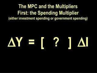
II. Multiplier Effect • ratio of a change in the equilibrium GDP to the change in (x) spending which caused it • change in real GDP / initial change in spending = the multiplier • Take our example from earlier: • $20 billion change in GDP / $5 increase in investment = Multiplier of 4
B. change is usually in investment (more volatile) -but can and will be applied to any component of AE C. “initial change in spending” is up or down shift of Agg. Expend schedule due to one of its components D. multiplies both negative and positive changes
E. Rationale of Multiplier • repetitive flow of expenditures of x are received as income by y • Change in income causes C and S to change in same direction ( as a fraction of the change in income) • Example: • Joe’s Business invests $5 b from ABC Machines • ABC Machines has $5 b in new income (they can C or S , based on MPC and MPS) (assume MPC = .75 in this example) • …so ABC Machines now adds $3.75 b in new Consumption • ….that $3.75 b is received as income by other firms and households (call them DEFG) and they can Consume .75 of that new income (= $2.81) • …..they spend $2.81 b and that is new income for firms and households (call them HIJK)….apply the MPC and now they can Consume $2.11 • ....and so on ….and so on…… • From the initial $5 b increase in Investment spending by Joe’s Business, the GDP equilibrium increased by $20 b.
F. Multiplier and MPS and MPC • Multiplier and MPS = inverse -The fraction of the additional income that is saved (MPS) determines the cumulative effects of additional spending Smaller MPS = larger multiplier -if less is Saved, then more is Consumed and more is added to GDP . if MPS = .25 or ¼ Multiplier = 4 if MPS = .33 or 1/3 Multiplier = 3 if MPS = .20 or 1/5 Multiplier = 5 2. Multiplier and MPC = direct -Larger MPC = larger multiplier if MPC = .75, then you know MPS = .25 (*MPS + MPC = 1) ….so you know Multiplier = 4 If MPC = .80, then you know MPS = .20 …so you know Multiplier =5
G. Formula for Multiplier • Since Multiplier is reciprocal of MPS….. Then….Multiplier = 1/MPS ….and since (MPC + MPS = 1)…then (1-MPC = MPS)….so…….. ….Multiplier also = 1/1-MPC
H. Significance of Multiplier • A small change in any component of AE can create a large change in GDP Equilibrium.
III. International Trade (Xn) and Government Spending (G) • *remember: back in Ch. 9, this model was a “private-closed” economy…..now with Xn and G it will be “mixed-open” • A. Open Economy (NET EXPORTS) • Net Exports and AE • X – M (Xn) • +Xn (X>M) shifts AE up (fig 10-4 on next slide) from C+I to C+I+Xn1 • –Xn (M>X) shifts AE down (fig 10-4 on next slide) from C+I to C+I+Xn2 • *assume for now that Xn is autonomous of GDP, like Investment)
B. Analyze effects of Xn on AE • Mulitiplier Effect • See on Figure 10-4 • Still assmue MPC = .75 and Multiplier = 4 • Just like a $5 b increase or decrease in Investment • When Xn increases by $5 b, it creates a $20 b increase in GDP Equilibrium • When Xn decreases by $5 b, it creates a $20 b decrease in GDP Equilibrium
C. Determinants of Xn • rising income of foreign nations = rising demand for US exports = rising GDP • foreign nations increase tariffs on US goods = less demand for US exports = lower GDP • depreciation of the US dollar = cheaper for foreign nations to buy US exports (and more expensive for US to buy foreign goods) = rising GDP
D. Public Sector: Government Spending (G) • G expenditures are subject to direct control. Manipulate them to offset overspending or overproduction to promote economic stability . • Assumptions: • I and Xn are independent of GDP • G expenditures do NOT stimulate private spending • G net tax revenues are from only personal taxes • fixed amount of taxes • P is constant
Basic applications: • adding G creates new, higher equilibrium at $550 (see table 10-3 and Figure 10-5 on next 2 slides) b. G expend are subject to the multiplier c. G expend is not financed by increased tax revenue (assume we operate on a balanced budget
IV. Tax 1. Lump Sum Tax a. Creates a reduction in DI (C+S) equal to amount of T b. Will reduce C and S : amount determined by MPC and MPS c. Tax will reduce C by an amount = T x MPC Ex: a $20 b lump sum tax will reduce DI by exactly $20 b ..BUT…..will only reduce C by $15 b if MPC = .75 {20 x .75 = 15} (also conclude that S declines by $5 b) 2. Tax and the Multiplier • $20 b T reduces C by $15 b • Remember …if MPC = .75 and MPS = .25…then Multiplier = 4 • ….so when C falls by $15 b; it will result in a $60 b decrease in GDP • ….so GDP Eq in Table 10-3 was $550 b …but now that T has been included, the new GDP Eq is $490 (see Table 10-4 and figure 10-6 on next 2 slides)
Figure 10-6 C+I+Xn+G 1 $20 b T = 15 b decrease in C C+I+Xn +G 2 490 550
V. Balanced Budget Multiplier = 1 AE 3 AE 1 AE 2 A. When G increases spending but wants to pay for it by increase T by exact amount (also works if G decreases spending and T) B. Keys G and T must go in same direction G and T must be same amount ------------------------------------ Find original Eq at $440 (AE 1) Apply a T increase of $10 b (shift to AE 2 ) (MPC = .80) = a C decrease of $8 b : ..so with a Multiplier of 5 ; creates a new Eq at $400 Apply increase in G of $10 b (Shift to AE 3 (with Multiplier of 5 ; creates new Eq at $450) Conclude: a.-compare original Eq at AE 1 and final Eq at AE 3 400 440 450 b.-GDP increase by $10 b ; the exact amount the G increased and the T increased c. -…so ….a G increase and a T increase of the same amount will create a GDP increase by exact amount of increased G…..so there is a Multiplier of 1….that is….The Balanced Budget Multiplier
Conclusion on Leakages and Injections • All Injections I + X(exports) + G • All Leakages S + M (imports) + T • When GDP is in Equilibrium…. I+X+G = S+M+T (Return to Table 10-4 – see row 7 with GDP $490)