Aggregate Expenditures
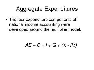
Aggregate Expenditures. The four expenditure components of national income accounting were developed around the multiplier model. AE = C + I + G + (X - IM). Expenditures Function. AE = C + I + G + (X - IM) AE o = autonomous expenditures that don’t change as income changes.

Aggregate Expenditures
E N D
Presentation Transcript
Aggregate Expenditures • The four expenditure components of national income accounting were developed around the multiplier model. AE = C + I + G + (X - IM)
Expenditures Function • AE = C + I + G + (X - IM) • AEo = autonomous expenditures that don’t change as income changes. • AE/ Y = those expenditures that change as income changes • We simplify the model for Econ 100: we pretend that only consumption changes when income changes.
The Marginal Propensity to Consume • The mpc is the fraction spent from an additional dollar of income.
Consumption and Income • Consumption depends on income. When income rises, consumption increases. • The marginal propensity to consume is the change in c divided by the change in y. • YD = C + S • MPC = C/YD • MPS = S/YD
Consumption and Saving • The MPC plus the MPS equals one. • To see why, note that, if you receive an additional $100 in disposable income, you will spend part of the income or not spend part of the income, that is save it. • In algebra: • C + S = YD.
The Marginal Propensity to Consume and AE • Since only consumption expenditures depend on income, in our simple model:
AE = aggregate expenditures AEo = autonomous expenditures mpc = marginal propensity to consume Y = income Expenditures Function • The expenditures function is expressed as a mathematical function: AE = AEo + mpcY
The Multiplier Equation • The multiplier is a number that reveals how much income will change in response to a change in autonomous expenditures. Multiplier = 1/(1 – mpc)
Alternative Equation • By definition: mpc + mps = 1 • Alternatively expressed: mps = 1 - mpc multiplier = 1/mps
The two equations Multiplier = 1/(1 – mpc) multiplier = 1/mps Because 1-mpc = mps What you don’t consume is what you save.
Real expenditures AE1 $4,210 30 AE0 4,090 1,052.5 30 1,022.5 $120 0 $4,090 $4,210 Real income An Upward Shift of AE, Fig. 10-8a, p 248
Aggregate production AE0 $4,152 AE1 30 4,062 30 1,412 1,382 $90 $4,062 $4,152 An Downward Shift of AE, Fig. 10-8b, p 248 Real expenditures 0 Real income
An Example of the Multiplier • Suppose Investment rises by $ 100 million • the mpc is .8 so the mps is .2 • Multiplier = 1/(1 – mpc) = 1/(1-.8) = 1/.2 = 5 • multiplier = 1/mps = 1/.2 = 10/2 = 5 • Rise in Equilibrium Income 5 * $100 = $500
Realistic Multipliers • Our simple model pretends that no one pays taxes and no one buys imports • We also assume that Investment and government spending don’t change when income changes. • The real multiplier is closer to 2 than to 5.
Realistic Multipliers • Observe that the multiplier is calculated assuming prices are not changing. • The multiplier tells us how much the AD curve shifts to the right. • When AD shifts, prices change so the change in equilibrium income is even less than an accurate multiplier predicts.